Plot of fitted curves
curvesplot.RdProvides a plot of all the fitted curves from a dataframe of the main workflow results, possibly extended with additional information (e.g. groups from functional annotation) used to color and/or split the curves.
Usage
curvesplot(extendedres, xmin = 0, xmax, y0shift = TRUE, scaling = TRUE,
                       facetby, facetby2, free.y.scales = FALSE, ncol4faceting,
                       colorby, removelegend = FALSE,
                        npoints = 500, line.size = 0.5,
                        line.alpha = 0.8, dose_log_transfo = FALSE,
                       addBMD = TRUE, BMDtype = c("zSD", "xfold"),
                       point.size = 1, point.alpha = 0.8)
Arguments
- extendedres
the dataframe of results provided by bmdcalc (res) or drcfit (fitres) or a subset of this data frame (selected lines). This dataframe can be extended with additional columns coming for example from the annotation of items, and some lines can be replicated if their corresponding item has more than one annotation. This extended dataframe must at least contain the column giving the identification of each curve (
id), the columnmodelnaming the fitted model and the values of the parameters (columnsb,c,d,e,f).- xmin
Minimal dose/concentration for definition of the x range (by default 0).
- xmax
Maximal dose/concentration for definition of the x range (can be defined as
max(f$omicdata$dose)withfthe output ofdrcfit()).- y0shift
If
TRUE(default choice) curves are all shifted to have the theoretical signal at the control at 0.- scaling
If
TRUE, deafult choice, curves are all shifted to have the theoretical signal at the control at 0y0and scaled by dividing by the maximal absolute signal change (up or down) from the signal at the controlmaxychange.- facetby
optional argument naming the column of
extendedreschosen to split the plot in facets (no split if omitted).- facetby2
optional argument naming the column of
extendedreschosen as an additional argument to split the plot in facets usingggplot2::facet_grid, with columns defined byfacetbyand rows defined byfacetby2(no split if omitted).- free.y.scales
if TRUE the y scales are free in the different facets.
- ncol4faceting
Number of columns for facetting (not used if
facetby2is also provided.- colorby
optional argument naming the column of
extendedreschosen to color the curves (no color if omitted).- removelegend
If
TRUEthe color legend is removed (useful if the number of colors is great).- npoints
Number of points computed on each curve to plot it.
- line.size
Width of the lines for plotting curves.
- line.alpha
Transparency of the lines for plotting curves.
- dose_log_transfo
If TRUE a log transformation of the dose is used in the plot. This option needs a definition of a strictly positive value of xmin in input.
- addBMD
If TRUE points are added on the curve at BMD-BMR values (requires to have BMD and BMD values in the first argument extendedres).
- BMDtype
The type of BMD to add,
"zSD"(default choice) or"xfold".- point.size
Size of the BMD-BMR points added on the curves.
- point.alpha
Transparency of the BMD-BMR points added on the curves.
Details
For each item of the extended dataframe, the name of the model
(column model) and the values of
the parameters (columns b, c, d, e, f)
are used to compute theoretical dose-response curves in the range
[xmin ; xmax].
See also
See plot.bmdboot.
Examples
# (1) A toy example on a very small subsample of a microarray data set)
#
datafilename <- system.file("extdata", "transcripto_very_small_sample.txt",
package = "DRomics")
o <- microarraydata(datafilename, check = TRUE, norm.method = "cyclicloess")
#> Just wait, the normalization using cyclicloess may take a few minutes.
s_quad <- itemselect(o, select.method = "quadratic", FDR = 0.01)
#> Removing intercept from test coefficients
f <- drcfit(s_quad, progressbar = TRUE)
#> The fitting may be long if the number of selected items is high.
#>
|
| | 0%
|
|==== | 6%
|
|======== | 12%
|
|============ | 18%
|
|================ | 24%
|
|===================== | 29%
|
|========================= | 35%
|
|============================= | 41%
|
|================================= | 47%
|
|===================================== | 53%
|
|========================================= | 59%
|
|============================================= | 65%
|
|================================================= | 71%
|
|====================================================== | 76%
|
|========================================================== | 82%
|
|============================================================== | 88%
|
|================================================================== | 94%
|
|======================================================================| 100%
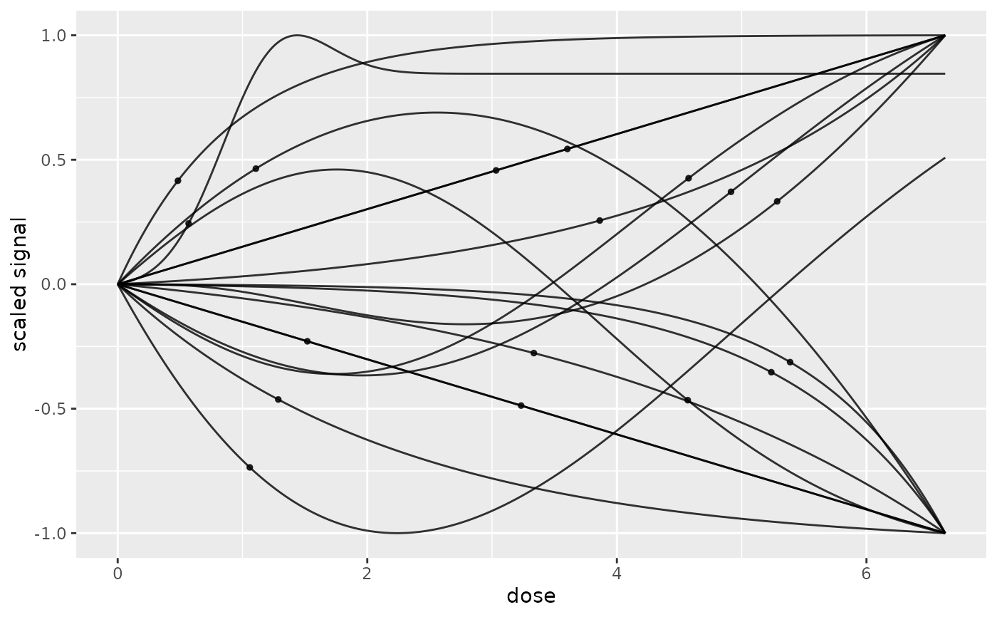
# (1.a)
# Default plot of all the curves
#
curvesplot(f$fitres, xmax = max(f$omicdata$dose), addBMD = FALSE)
 # \donttest{
# the equivalent using the output of bmdcalc
# which enables the add of BMD values
r <- bmdcalc(f)
curvesplot(r$res, xmax = max(f$omicdata$dose), addBMD = TRUE)
# \donttest{
# the equivalent using the output of bmdcalc
# which enables the add of BMD values
r <- bmdcalc(f)
curvesplot(r$res, xmax = max(f$omicdata$dose), addBMD = TRUE)
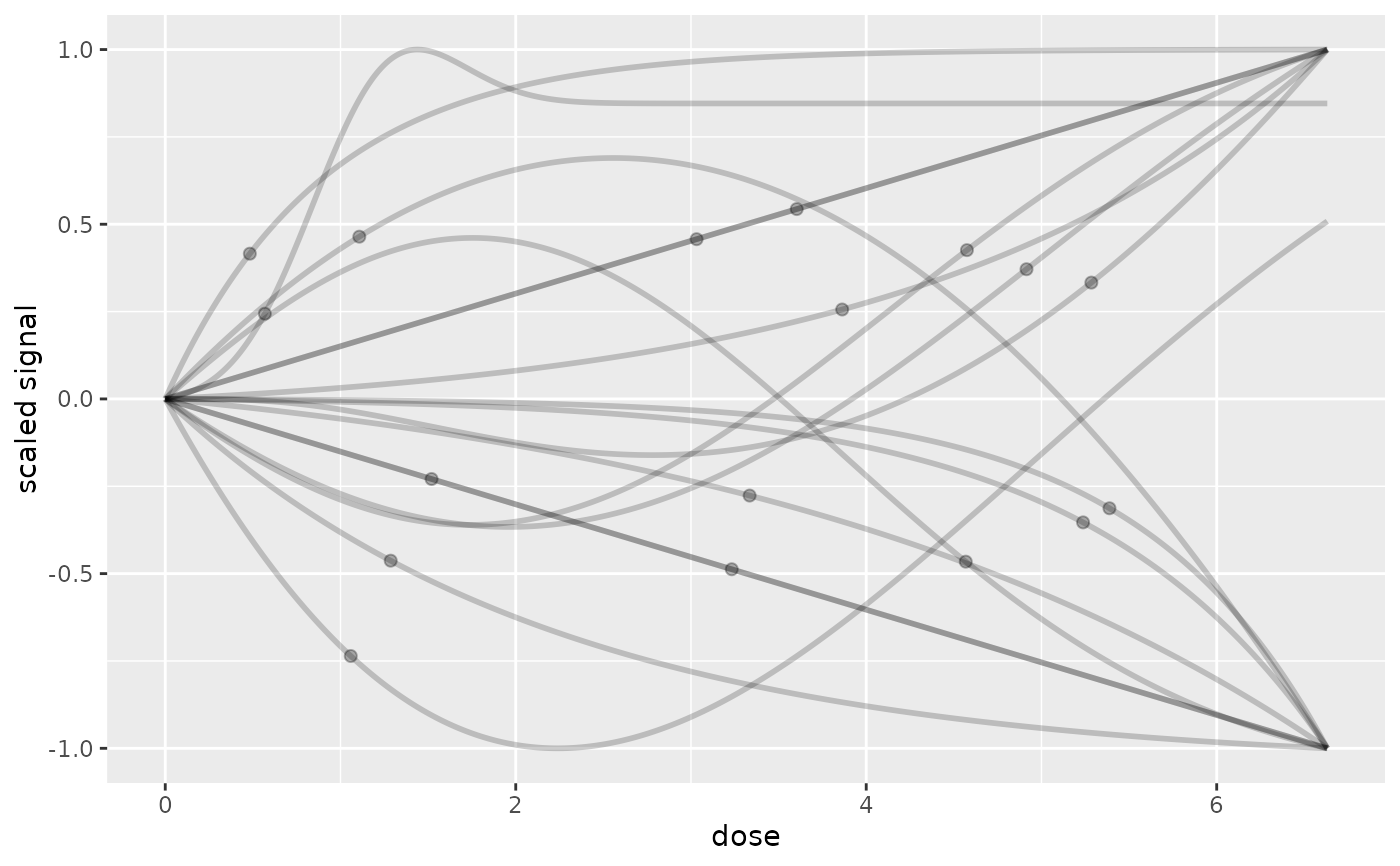
 # use of line size, point size, transparency
curvesplot(r$res, xmax = max(f$omicdata$dose),
line.alpha = 0.2, line.size = 1,
addBMD = TRUE, point.alpha = 0.3, point.size = 1.8)
# use of line size, point size, transparency
curvesplot(r$res, xmax = max(f$omicdata$dose),
line.alpha = 0.2, line.size = 1,
addBMD = TRUE, point.alpha = 0.3, point.size = 1.8)
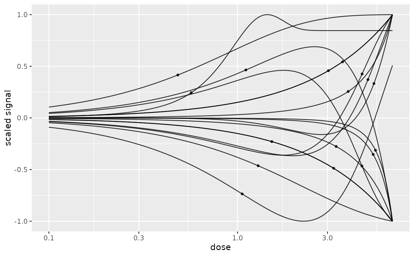
 # the same plot with dose in log scale (need xmin != 0 in input)
curvesplot(r$res, xmin = 0.1, xmax = max(f$omicdata$dose),
dose_log_transfo = TRUE, addBMD = TRUE)
# the same plot with dose in log scale (need xmin != 0 in input)
curvesplot(r$res, xmin = 0.1, xmax = max(f$omicdata$dose),
dose_log_transfo = TRUE, addBMD = TRUE)
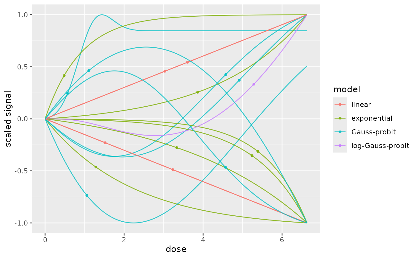
 # plot of curves colored by models
curvesplot(r$res, xmax = max(f$omicdata$dose), colorby = "model")
# plot of curves colored by models
curvesplot(r$res, xmax = max(f$omicdata$dose), colorby = "model")
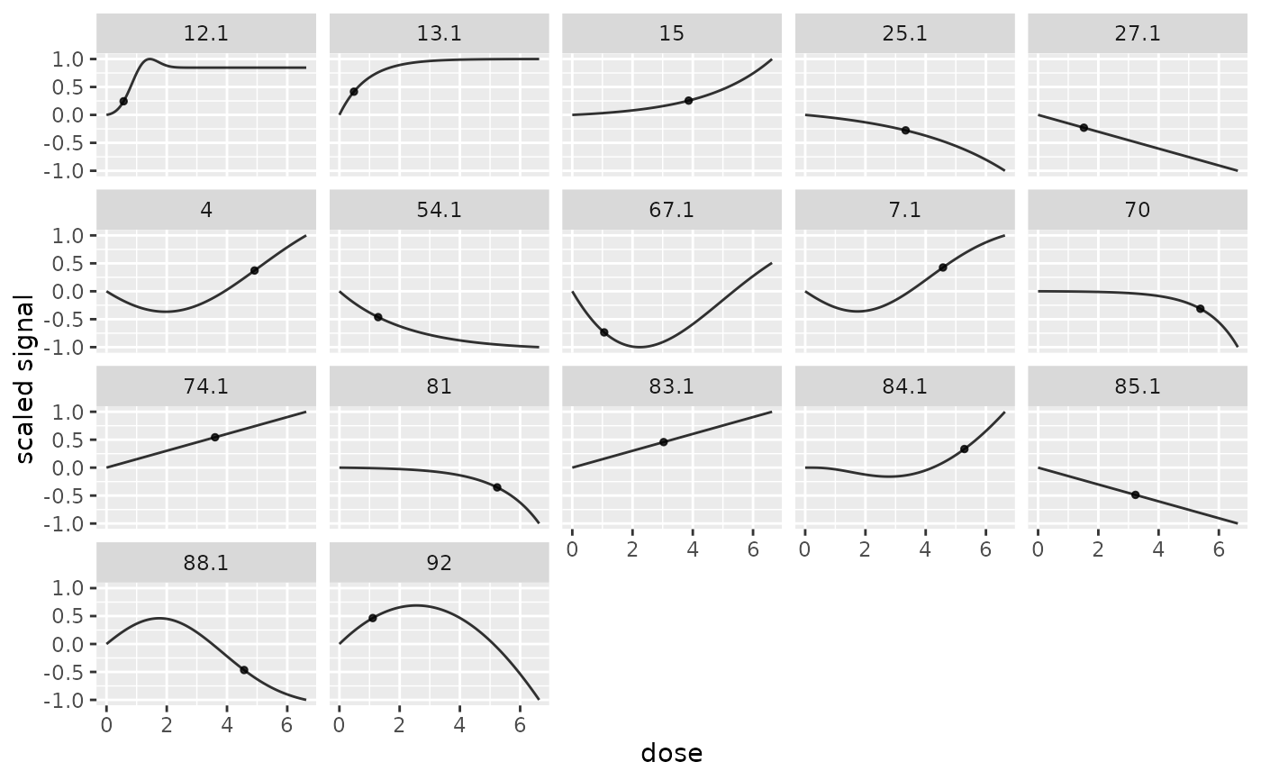
 # plot of curves facetted by item
curvesplot(r$res, xmax = max(f$omicdata$dose), facetby = "id")
# plot of curves facetted by item
curvesplot(r$res, xmax = max(f$omicdata$dose), facetby = "id")
 # plot of curves facetted by trends
curvesplot(r$res, xmax = max(f$omicdata$dose), facetby = "trend")
# plot of curves facetted by trends
curvesplot(r$res, xmax = max(f$omicdata$dose), facetby = "trend")
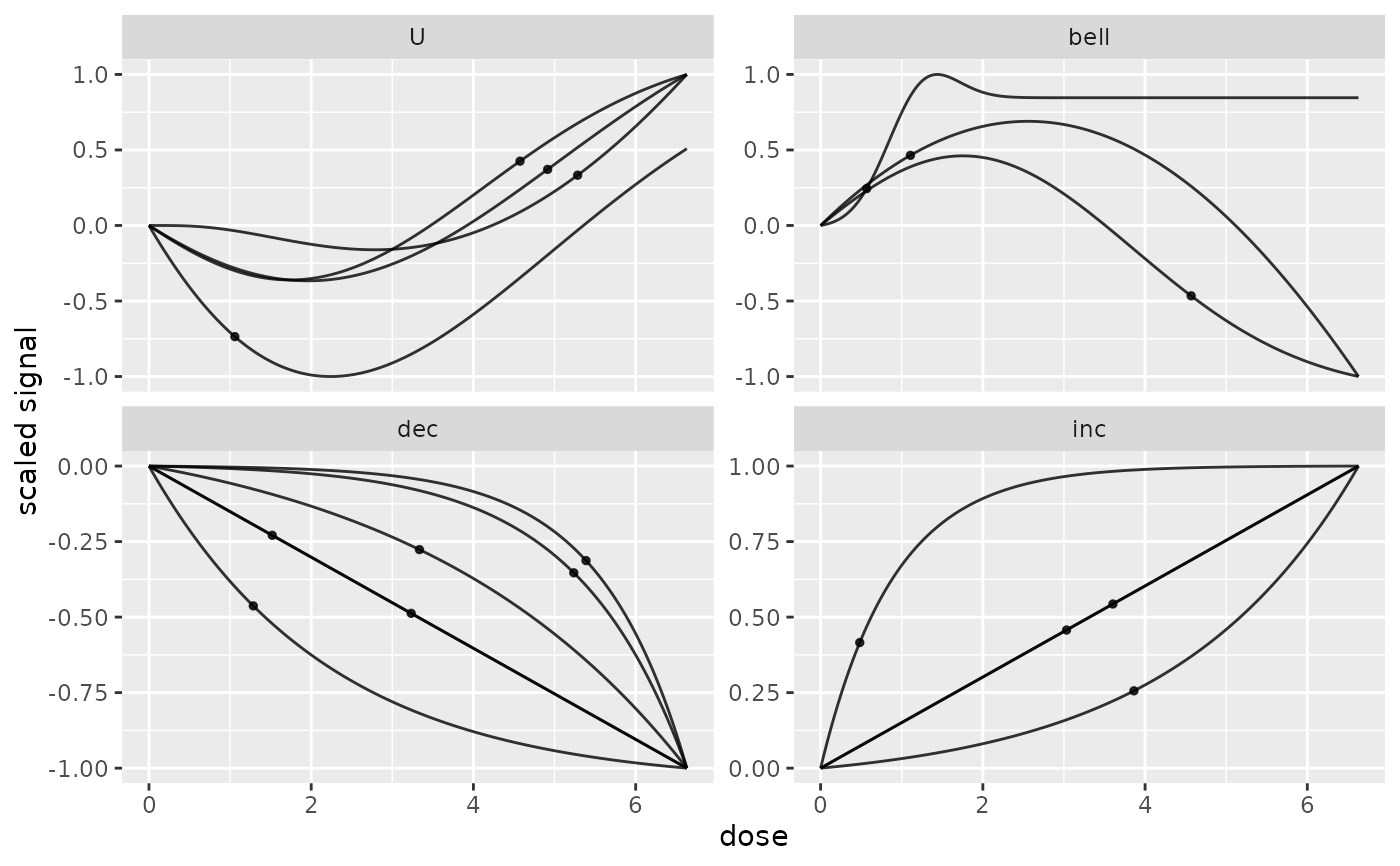
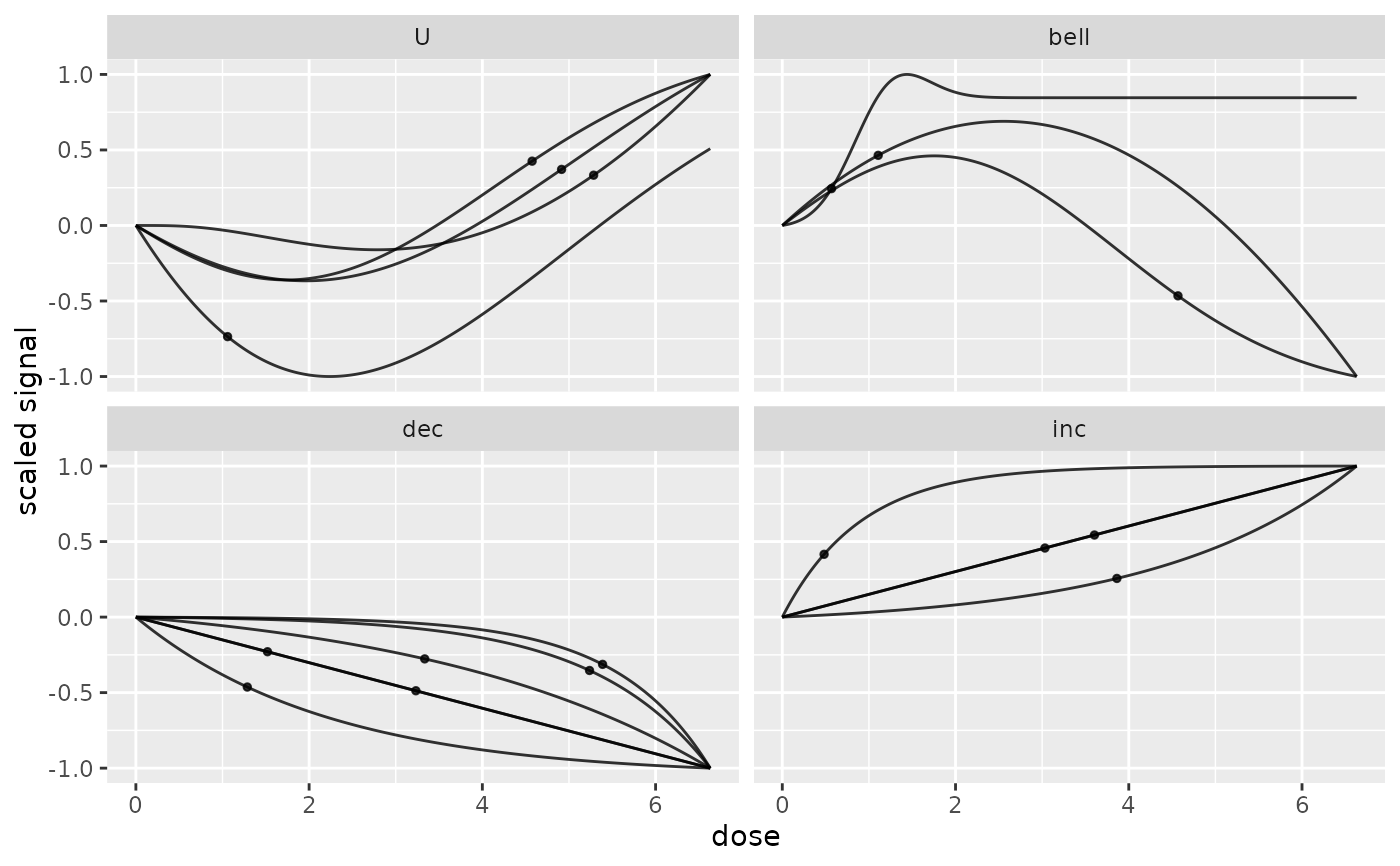 # the same plot with free y scales
curvesplot(r$res, xmax = max(f$omicdata$dose), facetby = "trend",
free.y.scales = TRUE)
# the same plot with free y scales
curvesplot(r$res, xmax = max(f$omicdata$dose), facetby = "trend",
free.y.scales = TRUE)
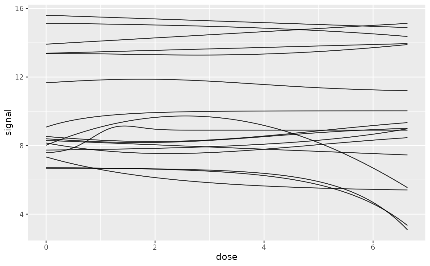
 # (1.b)
# Plot of all the curves without shifting y0 values to 0
# and without scaling
curvesplot(f$fitres, xmax = max(f$omicdata$dose), addBMD = FALSE,
scaling = FALSE, y0shift = FALSE)
# (1.b)
# Plot of all the curves without shifting y0 values to 0
# and without scaling
curvesplot(f$fitres, xmax = max(f$omicdata$dose), addBMD = FALSE,
scaling = FALSE, y0shift = FALSE)
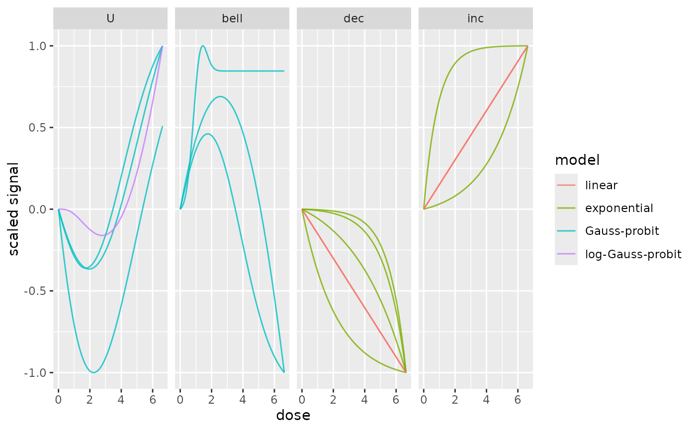
 # (1.c)
# Plot of all the curves colored by model, with one facet per trend
#
curvesplot(f$fitres, xmax = max(f$omicdata$dose), addBMD = FALSE,
facetby = "trend", colorby = "model")
# (1.c)
# Plot of all the curves colored by model, with one facet per trend
#
curvesplot(f$fitres, xmax = max(f$omicdata$dose), addBMD = FALSE,
facetby = "trend", colorby = "model")
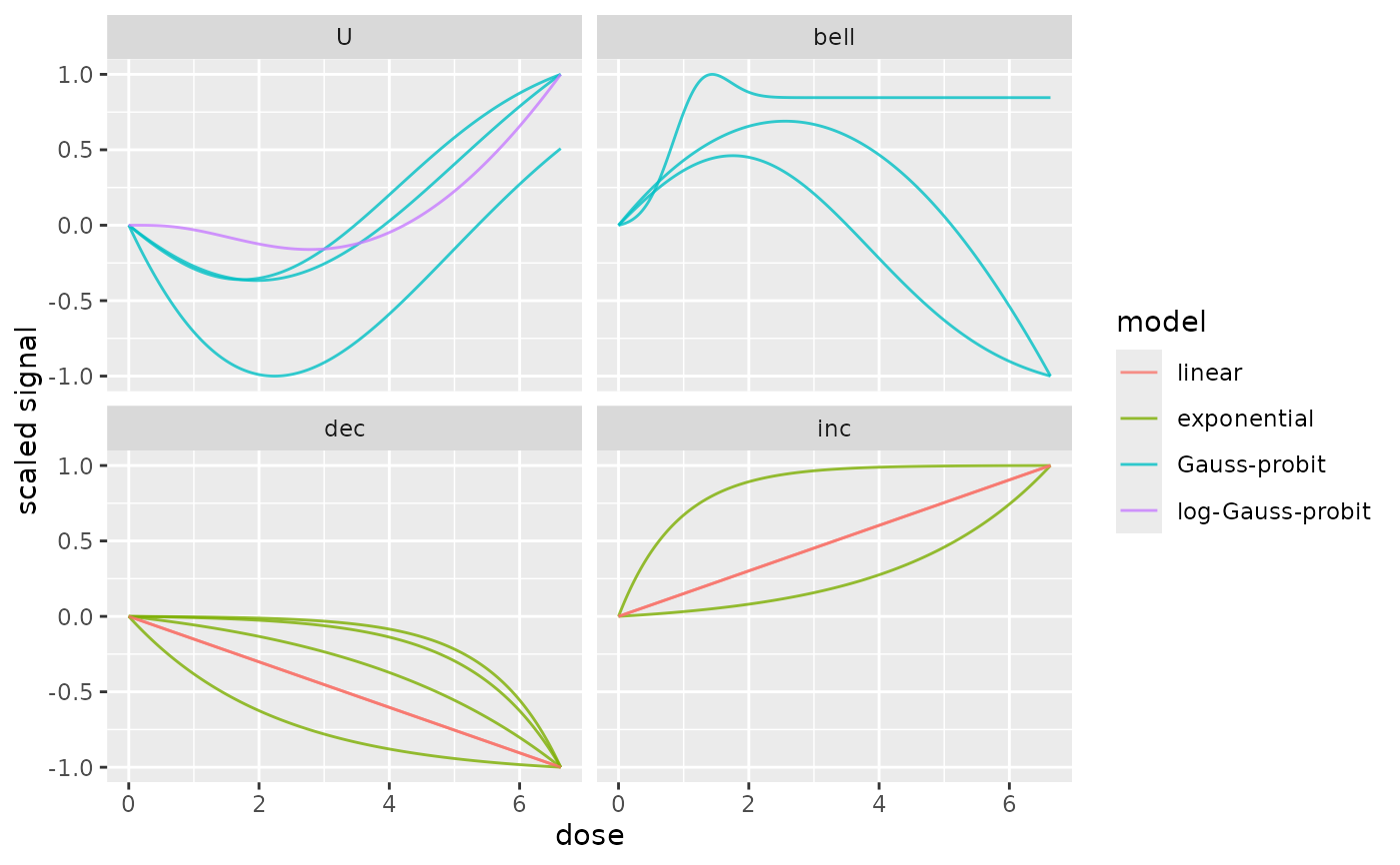
 # changing the number of columns
curvesplot(f$fitres, xmax = max(f$omicdata$dose), addBMD = FALSE,
facetby = "trend", colorby = "model", ncol4faceting = 4)
# changing the number of columns
curvesplot(f$fitres, xmax = max(f$omicdata$dose), addBMD = FALSE,
facetby = "trend", colorby = "model", ncol4faceting = 4)
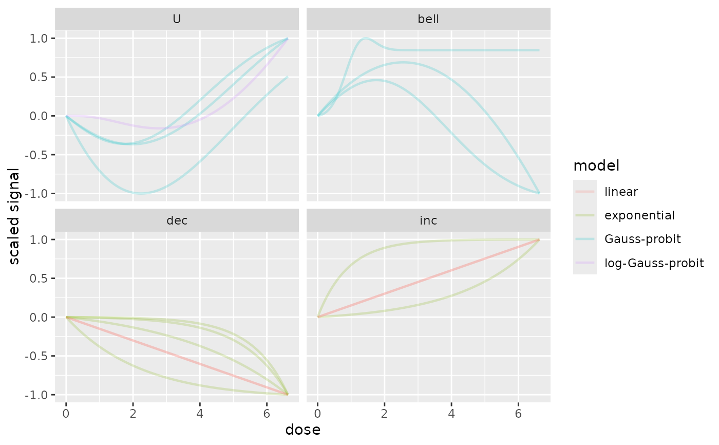
 # playing with size and transparency of lines
curvesplot(f$fitres, xmax = max(f$omicdata$dose), addBMD = FALSE,
facetby = "trend", colorby = "model",
line.size = 0.5, line.alpha = 0.8)
# playing with size and transparency of lines
curvesplot(f$fitres, xmax = max(f$omicdata$dose), addBMD = FALSE,
facetby = "trend", colorby = "model",
line.size = 0.5, line.alpha = 0.8)
 curvesplot(f$fitres, xmax = max(f$omicdata$dose), addBMD = FALSE,
facetby = "trend", colorby = "model",
line.size = 0.8, line.alpha = 0.2)
curvesplot(f$fitres, xmax = max(f$omicdata$dose), addBMD = FALSE,
facetby = "trend", colorby = "model",
line.size = 0.8, line.alpha = 0.2)
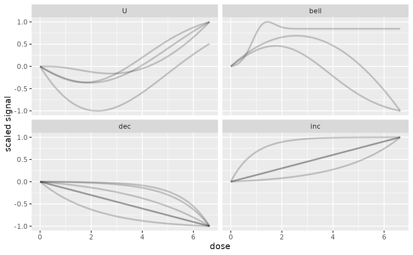
 curvesplot(f$fitres, xmax = max(f$omicdata$dose), addBMD = FALSE,
facetby = "trend", line.size = 1, line.alpha = 0.2)
curvesplot(f$fitres, xmax = max(f$omicdata$dose), addBMD = FALSE,
facetby = "trend", line.size = 1, line.alpha = 0.2)
 # (2) an example on a microarray data set (a subsample of a greater data set)
#
datafilename <- system.file("extdata", "transcripto_sample.txt", package="DRomics")
(o <- microarraydata(datafilename, check = TRUE, norm.method = "cyclicloess"))
#> Just wait, the normalization using cyclicloess may take a few minutes.
#> Elements of the experimental design in order to check the coding of the data:
#> Tested doses and number of replicates for each dose:
#>
#> 0 0.69 1.223 2.148 3.774 6.631
#> 5 5 5 5 5 5
#> Number of items: 1000
#> Identifiers of the first 20 items:
#> [1] "1" "2" "3" "4" "5.1" "5.2" "6.1" "6.2" "7.1" "7.2"
#> [11] "8.1" "8.2" "9.1" "9.2" "10.1" "10.2" "11.1" "11.2" "12.1" "12.2"
#> Data were normalized between arrays using the following method: cyclicloess
(s_quad <- itemselect(o, select.method = "quadratic", FDR = 0.001))
#> Removing intercept from test coefficients
#> Number of selected items using a quadratic trend test with an FDR of 0.001: 78
#> Identifiers of the first 20 most responsive items:
#> [1] "384.2" "383.1" "383.2" "384.1" "301.1" "363.1" "300.2" "364.2" "364.1"
#> [10] "363.2" "301.2" "300.1" "351.1" "350.2" "239.1" "240.1" "240.2" "370"
#> [19] "15" "350.1"
(f <- drcfit(s_quad, progressbar = TRUE))
#> The fitting may be long if the number of selected items is high.
#>
|
| | 0%
|
|= | 1%
|
|== | 3%
|
|=== | 4%
|
|==== | 5%
|
|==== | 6%
|
|===== | 8%
|
|====== | 9%
|
|======= | 10%
|
|======== | 12%
|
|========= | 13%
|
|========== | 14%
|
|=========== | 15%
|
|============ | 17%
|
|============= | 18%
|
|============= | 19%
|
|============== | 21%
|
|=============== | 22%
|
|================ | 23%
|
|================= | 24%
|
|================== | 26%
|
|=================== | 27%
|
|==================== | 28%
|
|===================== | 29%
|
|====================== | 31%
|
|====================== | 32%
|
|======================= | 33%
|
|======================== | 35%
|
|========================= | 36%
|
|========================== | 37%
|
|=========================== | 38%
|
|============================ | 40%
|
|============================= | 41%
|
|============================== | 42%
|
|=============================== | 44%
|
|=============================== | 45%
|
|================================ | 46%
|
|================================= | 47%
|
|================================== | 49%
|
|=================================== | 50%
|
|==================================== | 51%
|
|===================================== | 53%
|
|====================================== | 54%
|
|======================================= | 55%
|
|======================================= | 56%
|
|======================================== | 58%
|
|========================================= | 59%
|
|========================================== | 60%
|
|=========================================== | 62%
|
|============================================ | 63%
|
|============================================= | 64%
|
|============================================== | 65%
|
|=============================================== | 67%
|
|================================================ | 68%
|
|================================================ | 69%
|
|================================================= | 71%
|
|================================================== | 72%
|
|=================================================== | 73%
|
|==================================================== | 74%
|
|===================================================== | 76%
|
|====================================================== | 77%
|
|======================================================= | 78%
|
|======================================================== | 79%
|
|========================================================= | 81%
|
|========================================================= | 82%
|
|========================================================== | 83%
|
|=========================================================== | 85%
|
|============================================================ | 86%
|
|============================================================= | 87%
|
|============================================================== | 88%
|
|=============================================================== | 90%
|
|================================================================ | 91%
|
|================================================================= | 92%
|
|================================================================== | 94%
|
|================================================================== | 95%
|
|=================================================================== | 96%
|
|==================================================================== | 97%
|
|===================================================================== | 99%
|
|======================================================================| 100%
#> Results of the fitting using the AICc to select the best fit model
#> 11 dose-response curves out of 78 previously selected were removed
#> because no model could be fitted reliably.
#> Distribution of the chosen models among the 67 fitted dose-response curves:
#>
#> Hill linear exponential Gauss-probit
#> 0 11 30 23
#> log-Gauss-probit
#> 3
#> Distribution of the trends (curve shapes) among the 67 fitted dose-response curves:
#>
#> U bell dec inc
#> 6 20 22 19
(r <- bmdcalc(f))
#> 1 BMD-xfold values and 0 BMD-zSD values are not defined (coded NaN as
#> the BMR stands outside the range of response values defined by the model).
#> 28 BMD-xfold values and 0 BMD-zSD values could not be calculated (coded
#> NA as the BMR stands within the range of response values defined by the
#> model but outside the range of tested doses).
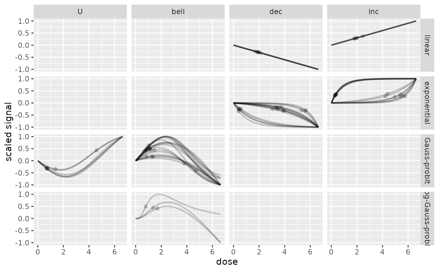
# plot split by trend and model with BMR-BMD points added on curves
# adding transparency
curvesplot(r$res, xmax = max(f$omicdata$dose),
line.alpha = 0.2, line.size = 0.8,
addBMD = TRUE, point.alpha = 0.2, point.size = 1.5,
facetby = "trend", facetby2 = "model")
# (2) an example on a microarray data set (a subsample of a greater data set)
#
datafilename <- system.file("extdata", "transcripto_sample.txt", package="DRomics")
(o <- microarraydata(datafilename, check = TRUE, norm.method = "cyclicloess"))
#> Just wait, the normalization using cyclicloess may take a few minutes.
#> Elements of the experimental design in order to check the coding of the data:
#> Tested doses and number of replicates for each dose:
#>
#> 0 0.69 1.223 2.148 3.774 6.631
#> 5 5 5 5 5 5
#> Number of items: 1000
#> Identifiers of the first 20 items:
#> [1] "1" "2" "3" "4" "5.1" "5.2" "6.1" "6.2" "7.1" "7.2"
#> [11] "8.1" "8.2" "9.1" "9.2" "10.1" "10.2" "11.1" "11.2" "12.1" "12.2"
#> Data were normalized between arrays using the following method: cyclicloess
(s_quad <- itemselect(o, select.method = "quadratic", FDR = 0.001))
#> Removing intercept from test coefficients
#> Number of selected items using a quadratic trend test with an FDR of 0.001: 78
#> Identifiers of the first 20 most responsive items:
#> [1] "384.2" "383.1" "383.2" "384.1" "301.1" "363.1" "300.2" "364.2" "364.1"
#> [10] "363.2" "301.2" "300.1" "351.1" "350.2" "239.1" "240.1" "240.2" "370"
#> [19] "15" "350.1"
(f <- drcfit(s_quad, progressbar = TRUE))
#> The fitting may be long if the number of selected items is high.
#>
|
| | 0%
|
|= | 1%
|
|== | 3%
|
|=== | 4%
|
|==== | 5%
|
|==== | 6%
|
|===== | 8%
|
|====== | 9%
|
|======= | 10%
|
|======== | 12%
|
|========= | 13%
|
|========== | 14%
|
|=========== | 15%
|
|============ | 17%
|
|============= | 18%
|
|============= | 19%
|
|============== | 21%
|
|=============== | 22%
|
|================ | 23%
|
|================= | 24%
|
|================== | 26%
|
|=================== | 27%
|
|==================== | 28%
|
|===================== | 29%
|
|====================== | 31%
|
|====================== | 32%
|
|======================= | 33%
|
|======================== | 35%
|
|========================= | 36%
|
|========================== | 37%
|
|=========================== | 38%
|
|============================ | 40%
|
|============================= | 41%
|
|============================== | 42%
|
|=============================== | 44%
|
|=============================== | 45%
|
|================================ | 46%
|
|================================= | 47%
|
|================================== | 49%
|
|=================================== | 50%
|
|==================================== | 51%
|
|===================================== | 53%
|
|====================================== | 54%
|
|======================================= | 55%
|
|======================================= | 56%
|
|======================================== | 58%
|
|========================================= | 59%
|
|========================================== | 60%
|
|=========================================== | 62%
|
|============================================ | 63%
|
|============================================= | 64%
|
|============================================== | 65%
|
|=============================================== | 67%
|
|================================================ | 68%
|
|================================================ | 69%
|
|================================================= | 71%
|
|================================================== | 72%
|
|=================================================== | 73%
|
|==================================================== | 74%
|
|===================================================== | 76%
|
|====================================================== | 77%
|
|======================================================= | 78%
|
|======================================================== | 79%
|
|========================================================= | 81%
|
|========================================================= | 82%
|
|========================================================== | 83%
|
|=========================================================== | 85%
|
|============================================================ | 86%
|
|============================================================= | 87%
|
|============================================================== | 88%
|
|=============================================================== | 90%
|
|================================================================ | 91%
|
|================================================================= | 92%
|
|================================================================== | 94%
|
|================================================================== | 95%
|
|=================================================================== | 96%
|
|==================================================================== | 97%
|
|===================================================================== | 99%
|
|======================================================================| 100%
#> Results of the fitting using the AICc to select the best fit model
#> 11 dose-response curves out of 78 previously selected were removed
#> because no model could be fitted reliably.
#> Distribution of the chosen models among the 67 fitted dose-response curves:
#>
#> Hill linear exponential Gauss-probit
#> 0 11 30 23
#> log-Gauss-probit
#> 3
#> Distribution of the trends (curve shapes) among the 67 fitted dose-response curves:
#>
#> U bell dec inc
#> 6 20 22 19
(r <- bmdcalc(f))
#> 1 BMD-xfold values and 0 BMD-zSD values are not defined (coded NaN as
#> the BMR stands outside the range of response values defined by the model).
#> 28 BMD-xfold values and 0 BMD-zSD values could not be calculated (coded
#> NA as the BMR stands within the range of response values defined by the
#> model but outside the range of tested doses).
# plot split by trend and model with BMR-BMD points added on curves
# adding transparency
curvesplot(r$res, xmax = max(f$omicdata$dose),
line.alpha = 0.2, line.size = 0.8,
addBMD = TRUE, point.alpha = 0.2, point.size = 1.5,
facetby = "trend", facetby2 = "model")
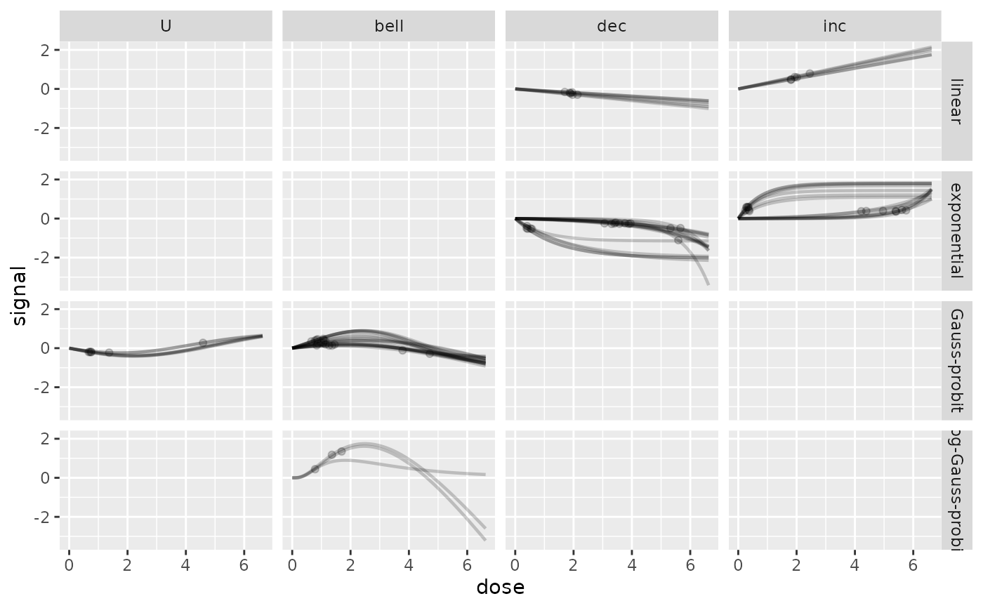
 # same plot without scaling
curvesplot(r$res, xmax = max(f$omicdata$dose),
line.alpha = 0.2, line.size = 0.8,
addBMD = TRUE, point.alpha = 0.2, point.size = 1.5,
scaling = FALSE, facetby = "trend", facetby2 = "model")
# same plot without scaling
curvesplot(r$res, xmax = max(f$omicdata$dose),
line.alpha = 0.2, line.size = 0.8,
addBMD = TRUE, point.alpha = 0.2, point.size = 1.5,
scaling = FALSE, facetby = "trend", facetby2 = "model")
 # (3) An example from data published by Larras et al. 2020
# in Journal of Hazardous Materials
# https://doi.org/10.1016/j.jhazmat.2020.122727
# a dataframe with metabolomic results (output $res of bmdcalc() or bmdboot() functions)
resfilename <- system.file("extdata", "triclosanSVmetabres.txt", package="DRomics")
res <- read.table(resfilename, header = TRUE, stringsAsFactors = TRUE)
str(res)
#> 'data.frame': 31 obs. of 27 variables:
#> $ id : Factor w/ 31 levels "NAP47_51","NAP_2",..: 2 3 4 5 6 7 8 9 10 11 ...
#> $ irow : int 2 21 28 34 38 47 49 51 53 67 ...
#> $ adjpvalue : num 6.23e-05 1.11e-05 1.03e-05 1.89e-03 4.16e-03 ...
#> $ model : Factor w/ 4 levels "Gauss-probit",..: 2 3 3 2 2 4 2 2 3 3 ...
#> $ nbpar : int 3 2 2 3 3 5 3 3 2 2 ...
#> $ b : num 0.4598 -0.0595 -0.0451 0.6011 0.6721 ...
#> $ c : num NA NA NA NA NA ...
#> $ d : num 5.94 5.39 7.86 6.86 6.21 ...
#> $ e : num -1.648 NA NA -0.321 -0.323 ...
#> $ f : num NA NA NA NA NA ...
#> $ SDres : num 0.126 0.0793 0.052 0.2338 0.2897 ...
#> $ typology : Factor w/ 10 levels "E.dec.concave",..: 2 7 7 2 2 9 2 2 7 7 ...
#> $ trend : Factor w/ 4 levels "U","bell","dec",..: 3 3 3 3 3 1 3 3 3 3 ...
#> $ y0 : num 5.94 5.39 7.86 6.86 6.21 ...
#> $ yrange : num 0.456 0.461 0.35 0.601 0.672 ...
#> $ maxychange : num 0.456 0.461 0.35 0.601 0.672 ...
#> $ xextrem : num NA NA NA NA NA ...
#> $ yextrem : num NA NA NA NA NA ...
#> $ BMD.zSD : num 0.528 1.333 1.154 0.158 0.182 ...
#> $ BMR.zSD : num 5.82 5.31 7.81 6.62 5.92 ...
#> $ BMD.xfold : num NA NA NA NA 0.832 ...
#> $ BMR.xfold : num 5.35 4.85 7.07 6.17 5.59 ...
#> $ BMD.zSD.lower : num 0.2001 0.8534 0.7519 0.0554 0.081 ...
#> $ BMD.zSD.upper : num 1.11 1.746 1.465 0.68 0.794 ...
#> $ BMD.xfold.lower : num Inf 7.611 Inf 0.561 0.329 ...
#> $ BMD.xfold.upper : num Inf Inf Inf Inf Inf ...
#> $ nboot.successful: int 957 1000 1000 648 620 872 909 565 1000 1000 ...
# a dataframe with annotation of each item identified in the previous file
# each item may have more than one annotation (-> more than one line)
annotfilename <- system.file("extdata", "triclosanSVmetabannot.txt", package="DRomics")
annot <- read.table(annotfilename, header = TRUE, stringsAsFactors = TRUE)
str(annot)
#> 'data.frame': 84 obs. of 2 variables:
#> $ metab.code: Factor w/ 31 levels "NAP47_51","NAP_2",..: 2 3 4 4 4 4 5 6 7 8 ...
#> $ path_class: Factor w/ 9 levels "Amino acid metabolism",..: 5 3 3 2 6 8 5 5 5 5 ...
# Merging of both previous dataframes
# in order to obtain an extenderes dataframe
# bootstrap results and annotation
extendedres <- merge(x = res, y = annot, by.x = "id", by.y = "metab.code")
head(extendedres)
#> id irow adjpvalue model nbpar b c d
#> 1 NAP47_51 46 7.158246e-04 linear 2 -0.05600559 NA 7.343571
#> 2 NAP_2 2 6.232579e-05 exponential 3 0.45981242 NA 5.941896
#> 3 NAP_23 21 1.106958e-05 linear 2 -0.05946618 NA 5.387252
#> 4 NAP_30 28 1.028343e-05 linear 2 -0.04507832 NA 7.859109
#> 5 NAP_30 28 1.028343e-05 linear 2 -0.04507832 NA 7.859109
#> 6 NAP_30 28 1.028343e-05 linear 2 -0.04507832 NA 7.859109
#> e f SDres typology trend y0 yrange maxychange
#> 1 NA NA 0.12454183 L.dec dec 7.343571 0.4346034 0.4346034
#> 2 -1.647958 NA 0.12604568 E.dec.convex dec 5.941896 0.4556672 0.4556672
#> 3 NA NA 0.07929266 L.dec dec 5.387252 0.4614576 0.4614576
#> 4 NA NA 0.05203245 L.dec dec 7.859109 0.3498078 0.3498078
#> 5 NA NA 0.05203245 L.dec dec 7.859109 0.3498078 0.3498078
#> 6 NA NA 0.05203245 L.dec dec 7.859109 0.3498078 0.3498078
#> xextrem yextrem BMD.zSD BMR.zSD BMD.xfold BMR.xfold BMD.zSD.lower
#> 1 NA NA 2.2237393 7.219029 NA 6.609214 0.9785095
#> 2 NA NA 0.5279668 5.815850 NA 5.347706 0.2000881
#> 3 NA NA 1.3334076 5.307960 NA 4.848527 0.8533711
#> 4 NA NA 1.1542677 7.807077 NA 7.073198 0.7518588
#> 5 NA NA 1.1542677 7.807077 NA 7.073198 0.7518588
#> 6 NA NA 1.1542677 7.807077 NA 7.073198 0.7518588
#> BMD.zSD.upper BMD.xfold.lower BMD.xfold.upper nboot.successful
#> 1 4.068699 Inf Inf 1000
#> 2 1.109559 Inf Inf 957
#> 3 1.746010 7.610936 Inf 1000
#> 4 1.464998 Inf Inf 1000
#> 5 1.464998 Inf Inf 1000
#> 6 1.464998 Inf Inf 1000
#> path_class
#> 1 Lipid metabolism
#> 2 Lipid metabolism
#> 3 Carbohydrate metabolism
#> 4 Carbohydrate metabolism
#> 5 Biosynthesis of other secondary metabolites
#> 6 Membrane transport
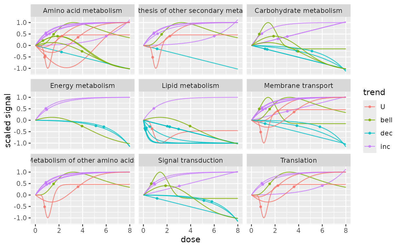
# Plot of the dose-response curves by pathway colored by trend
# with BMR-BMD points added on curves
curvesplot(extendedres, facetby = "path_class", npoints = 100, line.size = 0.5,
colorby = "trend", xmin = 0, xmax = 8, addBMD = TRUE)
# (3) An example from data published by Larras et al. 2020
# in Journal of Hazardous Materials
# https://doi.org/10.1016/j.jhazmat.2020.122727
# a dataframe with metabolomic results (output $res of bmdcalc() or bmdboot() functions)
resfilename <- system.file("extdata", "triclosanSVmetabres.txt", package="DRomics")
res <- read.table(resfilename, header = TRUE, stringsAsFactors = TRUE)
str(res)
#> 'data.frame': 31 obs. of 27 variables:
#> $ id : Factor w/ 31 levels "NAP47_51","NAP_2",..: 2 3 4 5 6 7 8 9 10 11 ...
#> $ irow : int 2 21 28 34 38 47 49 51 53 67 ...
#> $ adjpvalue : num 6.23e-05 1.11e-05 1.03e-05 1.89e-03 4.16e-03 ...
#> $ model : Factor w/ 4 levels "Gauss-probit",..: 2 3 3 2 2 4 2 2 3 3 ...
#> $ nbpar : int 3 2 2 3 3 5 3 3 2 2 ...
#> $ b : num 0.4598 -0.0595 -0.0451 0.6011 0.6721 ...
#> $ c : num NA NA NA NA NA ...
#> $ d : num 5.94 5.39 7.86 6.86 6.21 ...
#> $ e : num -1.648 NA NA -0.321 -0.323 ...
#> $ f : num NA NA NA NA NA ...
#> $ SDres : num 0.126 0.0793 0.052 0.2338 0.2897 ...
#> $ typology : Factor w/ 10 levels "E.dec.concave",..: 2 7 7 2 2 9 2 2 7 7 ...
#> $ trend : Factor w/ 4 levels "U","bell","dec",..: 3 3 3 3 3 1 3 3 3 3 ...
#> $ y0 : num 5.94 5.39 7.86 6.86 6.21 ...
#> $ yrange : num 0.456 0.461 0.35 0.601 0.672 ...
#> $ maxychange : num 0.456 0.461 0.35 0.601 0.672 ...
#> $ xextrem : num NA NA NA NA NA ...
#> $ yextrem : num NA NA NA NA NA ...
#> $ BMD.zSD : num 0.528 1.333 1.154 0.158 0.182 ...
#> $ BMR.zSD : num 5.82 5.31 7.81 6.62 5.92 ...
#> $ BMD.xfold : num NA NA NA NA 0.832 ...
#> $ BMR.xfold : num 5.35 4.85 7.07 6.17 5.59 ...
#> $ BMD.zSD.lower : num 0.2001 0.8534 0.7519 0.0554 0.081 ...
#> $ BMD.zSD.upper : num 1.11 1.746 1.465 0.68 0.794 ...
#> $ BMD.xfold.lower : num Inf 7.611 Inf 0.561 0.329 ...
#> $ BMD.xfold.upper : num Inf Inf Inf Inf Inf ...
#> $ nboot.successful: int 957 1000 1000 648 620 872 909 565 1000 1000 ...
# a dataframe with annotation of each item identified in the previous file
# each item may have more than one annotation (-> more than one line)
annotfilename <- system.file("extdata", "triclosanSVmetabannot.txt", package="DRomics")
annot <- read.table(annotfilename, header = TRUE, stringsAsFactors = TRUE)
str(annot)
#> 'data.frame': 84 obs. of 2 variables:
#> $ metab.code: Factor w/ 31 levels "NAP47_51","NAP_2",..: 2 3 4 4 4 4 5 6 7 8 ...
#> $ path_class: Factor w/ 9 levels "Amino acid metabolism",..: 5 3 3 2 6 8 5 5 5 5 ...
# Merging of both previous dataframes
# in order to obtain an extenderes dataframe
# bootstrap results and annotation
extendedres <- merge(x = res, y = annot, by.x = "id", by.y = "metab.code")
head(extendedres)
#> id irow adjpvalue model nbpar b c d
#> 1 NAP47_51 46 7.158246e-04 linear 2 -0.05600559 NA 7.343571
#> 2 NAP_2 2 6.232579e-05 exponential 3 0.45981242 NA 5.941896
#> 3 NAP_23 21 1.106958e-05 linear 2 -0.05946618 NA 5.387252
#> 4 NAP_30 28 1.028343e-05 linear 2 -0.04507832 NA 7.859109
#> 5 NAP_30 28 1.028343e-05 linear 2 -0.04507832 NA 7.859109
#> 6 NAP_30 28 1.028343e-05 linear 2 -0.04507832 NA 7.859109
#> e f SDres typology trend y0 yrange maxychange
#> 1 NA NA 0.12454183 L.dec dec 7.343571 0.4346034 0.4346034
#> 2 -1.647958 NA 0.12604568 E.dec.convex dec 5.941896 0.4556672 0.4556672
#> 3 NA NA 0.07929266 L.dec dec 5.387252 0.4614576 0.4614576
#> 4 NA NA 0.05203245 L.dec dec 7.859109 0.3498078 0.3498078
#> 5 NA NA 0.05203245 L.dec dec 7.859109 0.3498078 0.3498078
#> 6 NA NA 0.05203245 L.dec dec 7.859109 0.3498078 0.3498078
#> xextrem yextrem BMD.zSD BMR.zSD BMD.xfold BMR.xfold BMD.zSD.lower
#> 1 NA NA 2.2237393 7.219029 NA 6.609214 0.9785095
#> 2 NA NA 0.5279668 5.815850 NA 5.347706 0.2000881
#> 3 NA NA 1.3334076 5.307960 NA 4.848527 0.8533711
#> 4 NA NA 1.1542677 7.807077 NA 7.073198 0.7518588
#> 5 NA NA 1.1542677 7.807077 NA 7.073198 0.7518588
#> 6 NA NA 1.1542677 7.807077 NA 7.073198 0.7518588
#> BMD.zSD.upper BMD.xfold.lower BMD.xfold.upper nboot.successful
#> 1 4.068699 Inf Inf 1000
#> 2 1.109559 Inf Inf 957
#> 3 1.746010 7.610936 Inf 1000
#> 4 1.464998 Inf Inf 1000
#> 5 1.464998 Inf Inf 1000
#> 6 1.464998 Inf Inf 1000
#> path_class
#> 1 Lipid metabolism
#> 2 Lipid metabolism
#> 3 Carbohydrate metabolism
#> 4 Carbohydrate metabolism
#> 5 Biosynthesis of other secondary metabolites
#> 6 Membrane transport
# Plot of the dose-response curves by pathway colored by trend
# with BMR-BMD points added on curves
curvesplot(extendedres, facetby = "path_class", npoints = 100, line.size = 0.5,
colorby = "trend", xmin = 0, xmax = 8, addBMD = TRUE)
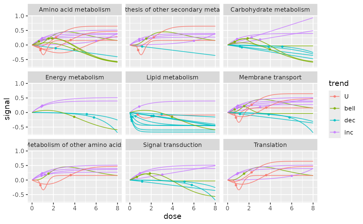
 # Plot of the dose-response curves without scaling, by pathway colored by trend
curvesplot(extendedres, facetby = "path_class", npoints = 100, line.size = 0.5,
colorby = "trend", scaling = FALSE, xmin = 0, xmax = 8)
# Plot of the dose-response curves without scaling, by pathway colored by trend
curvesplot(extendedres, facetby = "path_class", npoints = 100, line.size = 0.5,
colorby = "trend", scaling = FALSE, xmin = 0, xmax = 8)
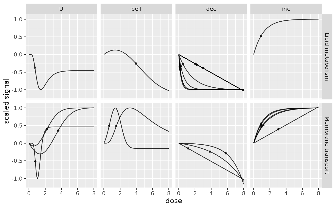
 # Plot of the dose-response curves split by pathway and by trend
# for a selection pathway
chosen_path_class <- c("Membrane transport", "Lipid metabolism")
ischosen <- is.element(extendedres$path_class, chosen_path_class)
curvesplot(extendedres[ischosen, ],
facetby = "trend", facetby2 = "path_class",
npoints = 100, line.size = 0.5, xmin = 0, xmax = 8)
# Plot of the dose-response curves split by pathway and by trend
# for a selection pathway
chosen_path_class <- c("Membrane transport", "Lipid metabolism")
ischosen <- is.element(extendedres$path_class, chosen_path_class)
curvesplot(extendedres[ischosen, ],
facetby = "trend", facetby2 = "path_class",
npoints = 100, line.size = 0.5, xmin = 0, xmax = 8)
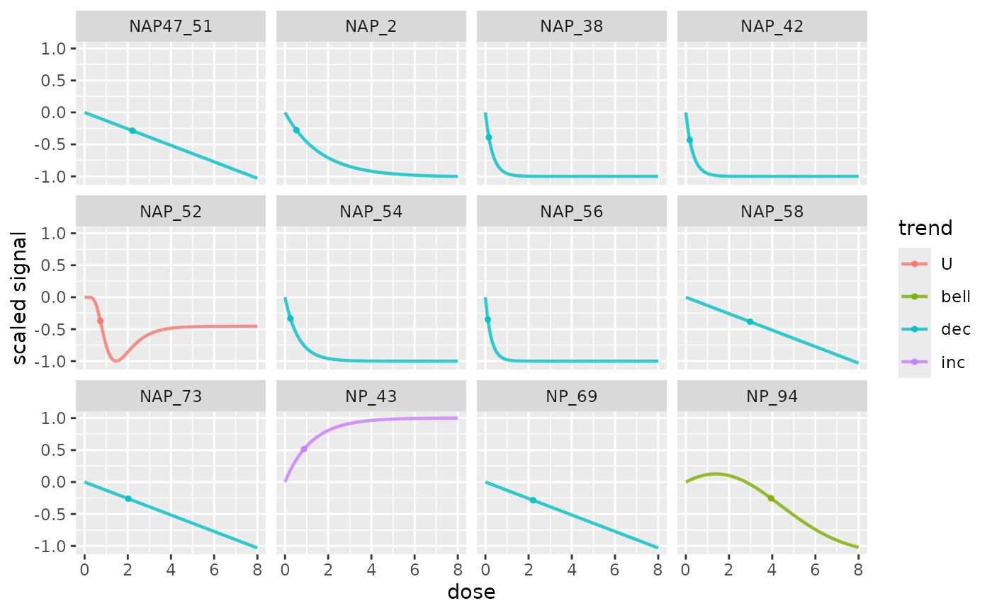
 # Plot of the dose-response curves for a specific pathway
# in this example the "lipid metabolism" pathclass
LMres <- extendedres[extendedres$path_class == "Lipid metabolism", ]
curvesplot(LMres, facetby = "id", npoints = 100, line.size = 0.8,
colorby = "trend", xmin = 0, xmax = 8)
# Plot of the dose-response curves for a specific pathway
# in this example the "lipid metabolism" pathclass
LMres <- extendedres[extendedres$path_class == "Lipid metabolism", ]
curvesplot(LMres, facetby = "id", npoints = 100, line.size = 0.8,
colorby = "trend", xmin = 0, xmax = 8)
 # }
# }