Dose response modelling for responsive items
drcfit.RdFits dose reponse models to responsive items.
Usage
drcfit(itemselect,
  information.criterion = c("AICc", "BIC", "AIC"),
  postfitfilter = TRUE, preventsfitsoutofrange = TRUE,
  enablesfequal0inGP = TRUE, enablesfequal0inLGP = TRUE,
  progressbar = TRUE, parallel = c("no", "snow", "multicore"), ncpus)

# S3 method for drcfit
print(x, ...)

# S3 method for drcfit
plot(x, items,
  plot.type = c("dose_fitted", "dose_residuals","fitted_residuals"),
  dose_log_transfo = TRUE, BMDoutput, BMDtype = c("zSD", "xfold"), ...)

plotfit2pdf(x, items,
  plot.type = c("dose_fitted", "dose_residuals", "fitted_residuals"),
  dose_log_transfo = TRUE, BMDoutput, BMDtype = c("zSD", "xfold"),
  nrowperpage = 6, ncolperpage = 4, path2figs = getwd())
Arguments
- itemselect
An object of class
"itemselect"returned by the functionitemselect.- information.criterion
The information criterion used to select the best fit model,
"AICc"as recommended and default choice (the corrected version of the AIC that is recommended for small samples (see Burnham and Anderson 2004),"BIC"or"AIC".- postfitfilter
If
TRUEfits with significant trends on residuals (showing a global significant quadratic trend of the residuals as a function of the dose (in rank-scale)) are considered as failures and so eliminated. It is strongly recommended to let it atTRUE, its default value.- preventsfitsoutofrange
If
TRUEfits of Gaussian or log-Gaussian models that give an extremum value outside the range of the observed signal for an item are eliminated from the candidate models for this item, before the choice of the best. It is strongly recommended to let it atTRUE, its default value.- enablesfequal0inGP
If
TRUEwhen the fit of a Gauss-probit model with 5 parameters is successful, its simplified version withf = 0is also fitted and included in the candidate models. This submodel of the log-Gauss-probit model corresponds to the probit model. We recommend to let this argument atTRUE, its default value, in order to prevent overfitting, and prefer the description of a monotonic curve when the parameter f is not necessary to model the data according to the information criterion.- enablesfequal0inLGP
If
TRUEwhen the fit of a log-Gauss-probit model with 5 parameters is successful, its simplified version withf = 0is also fitted and included in the candidate models. This submodel of the log-Gauss-probit model corresponds to the log-probit model. We recommend to let this argument atTRUE, its default value, in order to prevent overfitting and prefer the description of a monotonic curve when the parameter f is not necessary to model the data according to the information criterion.- progressbar
If
TRUEa progress bar is used to follow the fitting process.- parallel
The type of parallel operation to be used,
"snow"or"multicore"(the second one not being available on Windows), or"no"if no parallel operation.- ncpus
Number of processes to be used in parallel operation : typically one would fix it to the number of available CPUs.
- x
An object of class
"drcfit".- items
Argument of the
plot.drcfitfunction : the number of the first fits to plot (20 items max) or the character vector specifying the identifiers of the items to plot (20 items max).- plot.type
The type of plot, by default
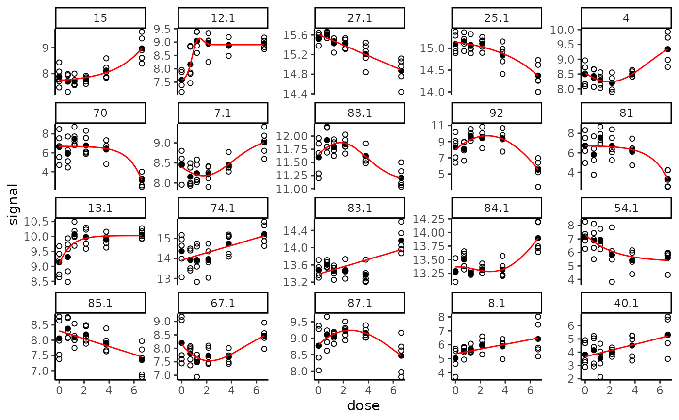
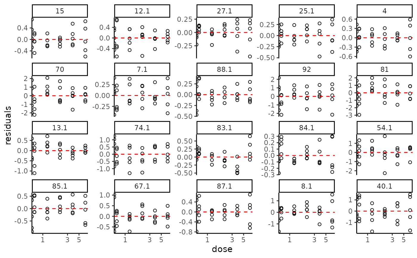
"dose_fitted"for the plot of fitted curves with the observed points added to the plot and the observed means at each dose added as black plain circles,"dose_residuals"for the plot of the residuals as function of the dose, and"fitted_residuals"for the plot of the residuals as function of the fitted value.- dose_log_transfo
By default at
TRUEto use a log transformation for the dose axis (only used if the dose is in x-axis, so not forplot.type"fitted_residuals").- BMDoutput
Argument that can be used to add BMD values and optionally their confidence intervals on a plot of type
"dose_fitted". To do that you must previously applybmdcalcand optionallybmdbootonxof classdrcfitand then give in this argument the output ofbmdcalcorbmdboot.- BMDtype
The type of BMD to add on the plot,
"zSD"(default choice) or"xfold"(only used if BMDoutput is not missing).- nrowperpage
Number of rows of plots when plots are saved in a pdf file using plotfit2pdf() (passed to
facet_wrap()).- ncolperpage
Number of columns of plots when plots are saved in a pdf file using plotfit2pdf() (passed to
facet_wrap()).- path2figs
File path when plots are saved in a pdf file using plotfit2pdf()
- ...
Further arguments passed to graphical or print functions.
Details
For each selected item, five dose-response models (linear, Hill, exponential,
Gauss-probit and log-Gauss-probit, see Larras et al. 2018
for their definition) are fitted by non linear regression,
using the nls function. If a fit of a biphasic model gives a extremum
value out of the range of the observed signal, it is eliminated (this may happen in rare cases,
especially on observational data when the number of samples is high and the dose in uncontrolled,
if doses are not distributed all along the dose range).
The best fit is chosen as the one giving the lowest AICc
(or BIC or AIC) value. The use of the AICc (second-order Akaike criterion)
instead of the AIC
is strongly recommended to prevent the overfitting that may occur with dose-response designs
with a small number of data points (Hurvich and Tsai, 1989; Burnham and Anderson DR, 2004).
Note that in the extremely rare cases where the number of
data points would be great, the AIC would converge to the AICc and both procedures would be equivalent.
Items with the best AICc value not lower than the AICc value of the null model (constant model) minus 2
are eliminated. Items with the best fit showing a global significant quadratic trend of the residuals
as a function of the dose (in rank-scale) are also eliminated (the best fit is considered as
not reliable in such cases).
Each retained item is classified in four classes by its global trend, which can be used to roughly describe the shape of each dose-response curve:
inc for increasing curves,
dec for decreasing curves ,
U for U-shape curves,
bell for bell-shape curves.
Some curves fitted by a Gauss-probit model can be classified as increasing or decreasing when the
dose value at which their extremum is reached is at zero or if their simplified version with f = 0
is retained (corresponding to the probit model).
Some curves fitted by a log-Gauss-probit model can be classified as increasing or decreasing
if their simplified version with f = 0
is retained (corresponding to the log-probit model).
Each retained item is thus classified in a 16 class typology depending of the chosen model and of its parameter values :
H.inc for increasing Hill curves,
H.dec for decreasing Hill curves,
L.inc for increasing linear curves,
L.dec for decreasing linear curves,
E.inc.convex for increasing convex exponential curves,
E.dec.concave for decreasing concave exponential curves,
E.inc.concave for increasing concave exponential curves,
E.dec.convex for decreasing convex exponential curves,
GP.U for U-shape Gauss-probit curves,
GP.bell for bell-shape Gauss-probit curves,
GP.inc for increasing Gauss-probit curves,
GP.dec for decreasing Gauss-probit curves,
lGP.U for U-shape log-Gauss-probit curves,
lGP.bell for bell-shape log-Gauss-probit curves.
lGP.inc for increasing log-Gauss-probit curves,
lGP.dec for decreasing log-Gauss-probit curves,
Value
drcfit returns an object of class "drcfit", a list with 4 components:
- fitres
a data frame reporting the results of the fit on each selected item for which a successful fit is reached (one line per item) sorted in the ascending order of the adjusted p-values returned by function
itemselect. The different columns correspond to the identifier of each item (id), the row number of this item in the initial data set (irow), the adjusted p-value of the selection step (adjpvalue), the name of the best fit model (model), the number of fitted parameters (nbpar), the values of the parametersb,c,d,eandf, (NAfor non used parameters), the residual standard deviation (SDres), the typology of the curve (typology), the rough trend of the curve (trend) defined with four classes (U, bell, increasing or decreasing shape), the theoretical y value at the controly0), the theoretical y value at the maximal doseyatdosemax), the theoretical y range for x within the range of tested doses (yrange), the maximal absolute y change (up or down) from the control(maxychange) and for biphasic curves the x value at which their extremum is reached (xextrem) and the corresponding y value (yextrem).- omicdata
The object containing all the data, as given in input of
itemselect()which is also a component of the output ofitemselect().- information.criterion
The information criterion used to select the best fit model as given in input.
- information.criterion.val
A data frame reporting the IC values (AICc, BIC or AIC) values for each selected item (one line per item) and each fitted model (one colum per model with the IC value fixed at
Infwhen the fit failed).- n.failure
The number of previously selected items on which the workflow failed to fit an acceptable model.
- unfitres
A data frame reporting the results on each selected item for which no successful fit is reached (one line per item) sorted in the ascending order of the adjusted p-values returned by function
itemselect. The different columns correspond to the identifier of each item (id), the row number of this item in the initial data set (irow), the adjusted p-value of the selection step (adjpvalue), and code for the reason of the fitting failure (cause, equal to"constant.model"if the best fit model is a constant model or"trend.in.residuals"if the best fit model is rejected due to quadratic trend on residuals.)- residualtests
A data frame of P-values of the tests performed on residuals, on the mean trend (
resimeantrendP) and on the variance trend (resivartrendP). The first one tests a global significant quadratic trend of the residuals as a function of the dose in rank-scale (used to eliminate unreliable fits) and the second one a global significant quadratic trend of the residuals in absolute value as a function of the dose in rank-scale (used to alert in case of heteroscedasticity).
See also
See nls for details about the non linear regression function and
targetplot to plot target items (even if non responsive or unfitted).
References
Burnham, KP, Anderson DR (2004). Multimodel inference: understanding AIC and BIC in model selection. Sociological methods & research, 33(2), 261-304.
Hurvich, CM, Tsai, CL (1989). Regression and time series model selection in small samples. Biometrika, 76(2), 297-307.
Larras F, Billoir E, Baillard V, Siberchicot A, Scholz S, Wubet T, Tarkka M, Schmitt-Jansen M and Delignette-Muller ML (2018). DRomics: a turnkey tool to support the use of the dose-response framework for omics data in ecological risk assessment. Environmental science & technology.doi:10.1021/acs.est.8b04752
Examples
# (1) a toy example (a very small subsample of a microarray data set)
#
datafilename <- system.file("extdata", "transcripto_very_small_sample.txt", package = "DRomics")
# to test the package on a small (for a quick calculation) but not very small data set
# use the following commented line
# datafilename <- system.file("extdata", "transcripto_sample.txt", package = "DRomics")
o <- microarraydata(datafilename, check = TRUE, norm.method = "cyclicloess")
#> Just wait, the normalization using cyclicloess may take a few minutes.
s_quad <- itemselect(o, select.method = "quadratic", FDR = 0.05)
#> Removing intercept from test coefficients
(f <- drcfit(s_quad, progressbar = TRUE))
#> The fitting may be long if the number of selected items is high.
#>
|
| | 0%
|
|=== | 5%
|
|======= | 10%
|
|========== | 14%
|
|============= | 19%
|
|================= | 24%
|
|==================== | 29%
|
|======================= | 33%
|
|=========================== | 38%
|
|============================== | 43%
|
|================================= | 48%
|
|===================================== | 52%
|
|======================================== | 57%
|
|=========================================== | 62%
|
|=============================================== | 67%
|
|================================================== | 71%
|
|===================================================== | 76%
|
|========================================================= | 81%
|
|============================================================ | 86%
|
|=============================================================== | 90%
|
|=================================================================== | 95%
|
|======================================================================| 100%
#> Results of the fitting using the AICc to select the best fit model
#> 1 dose-response curves out of 21 previously selected were removed
#> because no model could be fitted reliably.
#> Distribution of the chosen models among the 20 fitted dose-response curves:
#>
#> Hill linear exponential Gauss-probit
#> 0 6 6 7
#> log-Gauss-probit
#> 1
#> Distribution of the trends (curve shapes) among the 20 fitted dose-response curves:
#>
#> U bell dec inc
#> 4 4 6 6
# Default plot
plot(f)
#> Warning: Transformation introduced infinite values in continuous x-axis
#> Warning: Transformation introduced infinite values in continuous x-axis
#> Warning: Transformation introduced infinite values in continuous x-axis
 # \donttest{
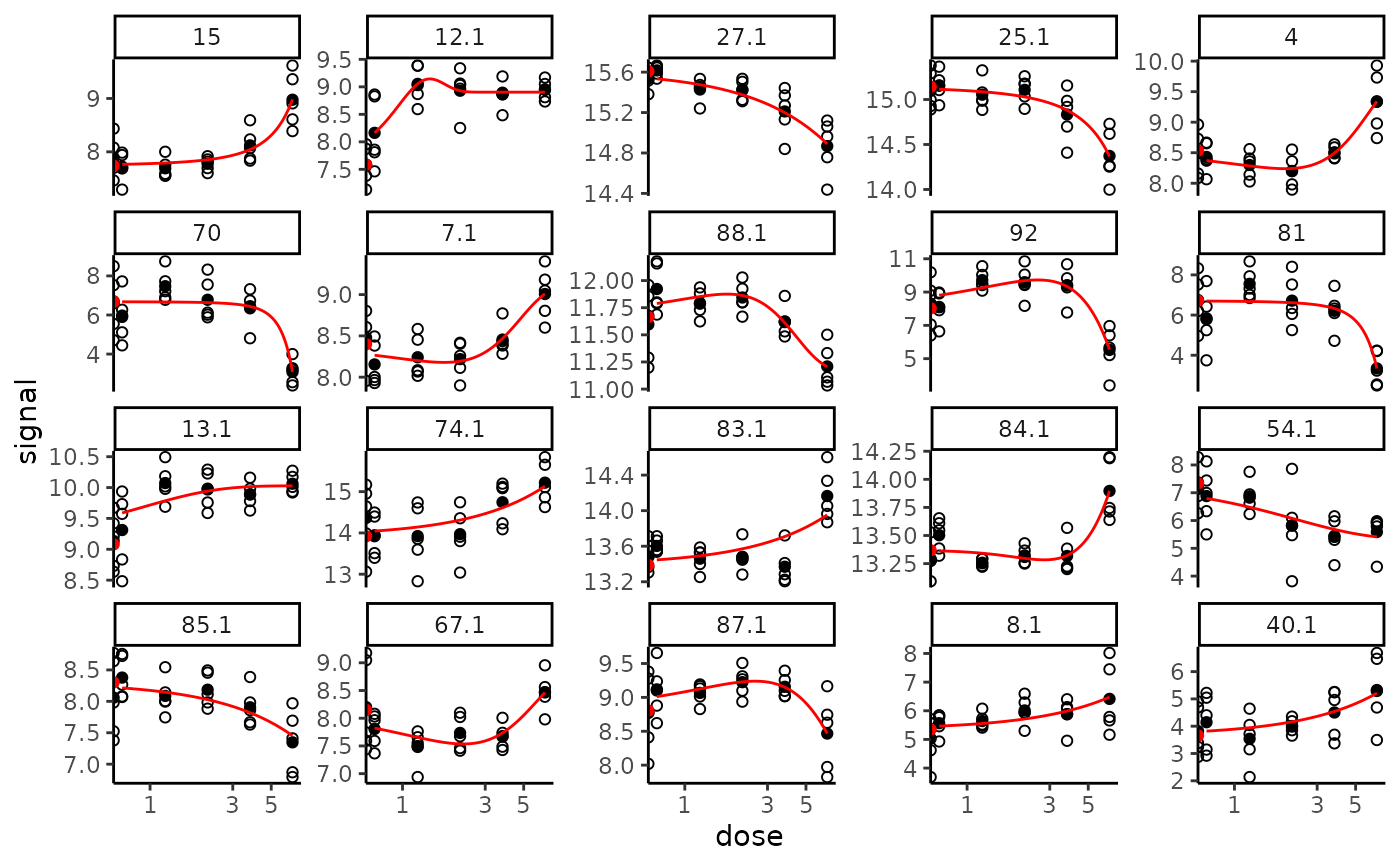
# The same plot without log transformation of the doses
# (in raw scale of doses)
plot(f, dose_log_transfo = FALSE)
# \donttest{
# The same plot without log transformation of the doses
# (in raw scale of doses)
plot(f, dose_log_transfo = FALSE)
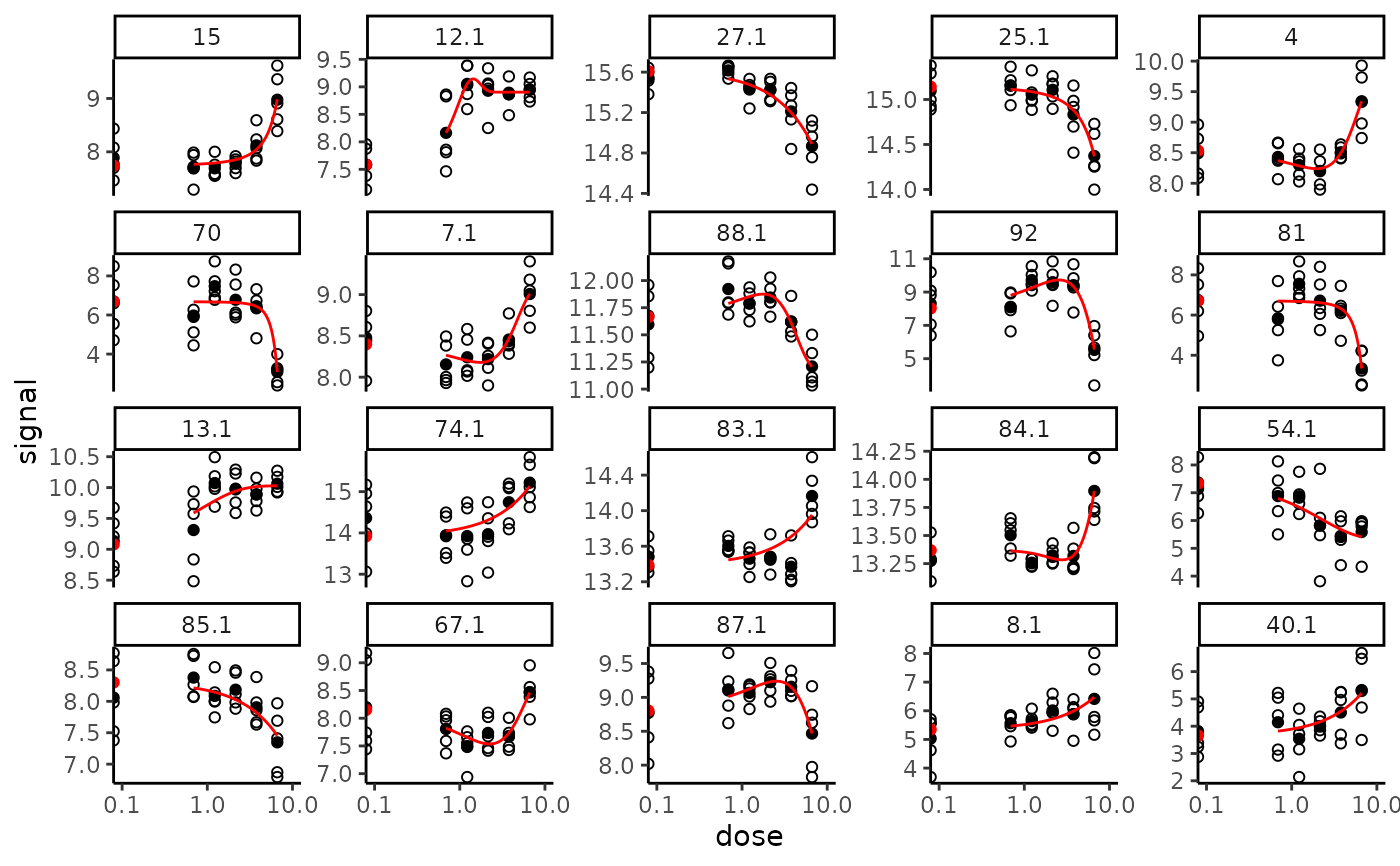
 # The same plot in x log scale choosing x limits for plot
if (require(ggplot2))
plot(f, dose_log_transfo = TRUE) +
scale_x_log10(limits = c(0.1, 10))
#> Warning: Transformation introduced infinite values in continuous x-axis
#> Warning: Transformation introduced infinite values in continuous x-axis
#> Warning: Transformation introduced infinite values in continuous x-axis
#> Scale for x is already present.
#> Adding another scale for x, which will replace the existing scale.
# The same plot in x log scale choosing x limits for plot
if (require(ggplot2))
plot(f, dose_log_transfo = TRUE) +
scale_x_log10(limits = c(0.1, 10))
#> Warning: Transformation introduced infinite values in continuous x-axis
#> Warning: Transformation introduced infinite values in continuous x-axis
#> Warning: Transformation introduced infinite values in continuous x-axis
#> Scale for x is already present.
#> Adding another scale for x, which will replace the existing scale.
 #> Warning: Transformation introduced infinite values in continuous x-axis
#> Warning: Transformation introduced infinite values in continuous x-axis
#> Warning: Transformation introduced infinite values in continuous x-axis
#> Warning: Transformation introduced infinite values in continuous x-axis
#> Warning: Transformation introduced infinite values in continuous x-axis
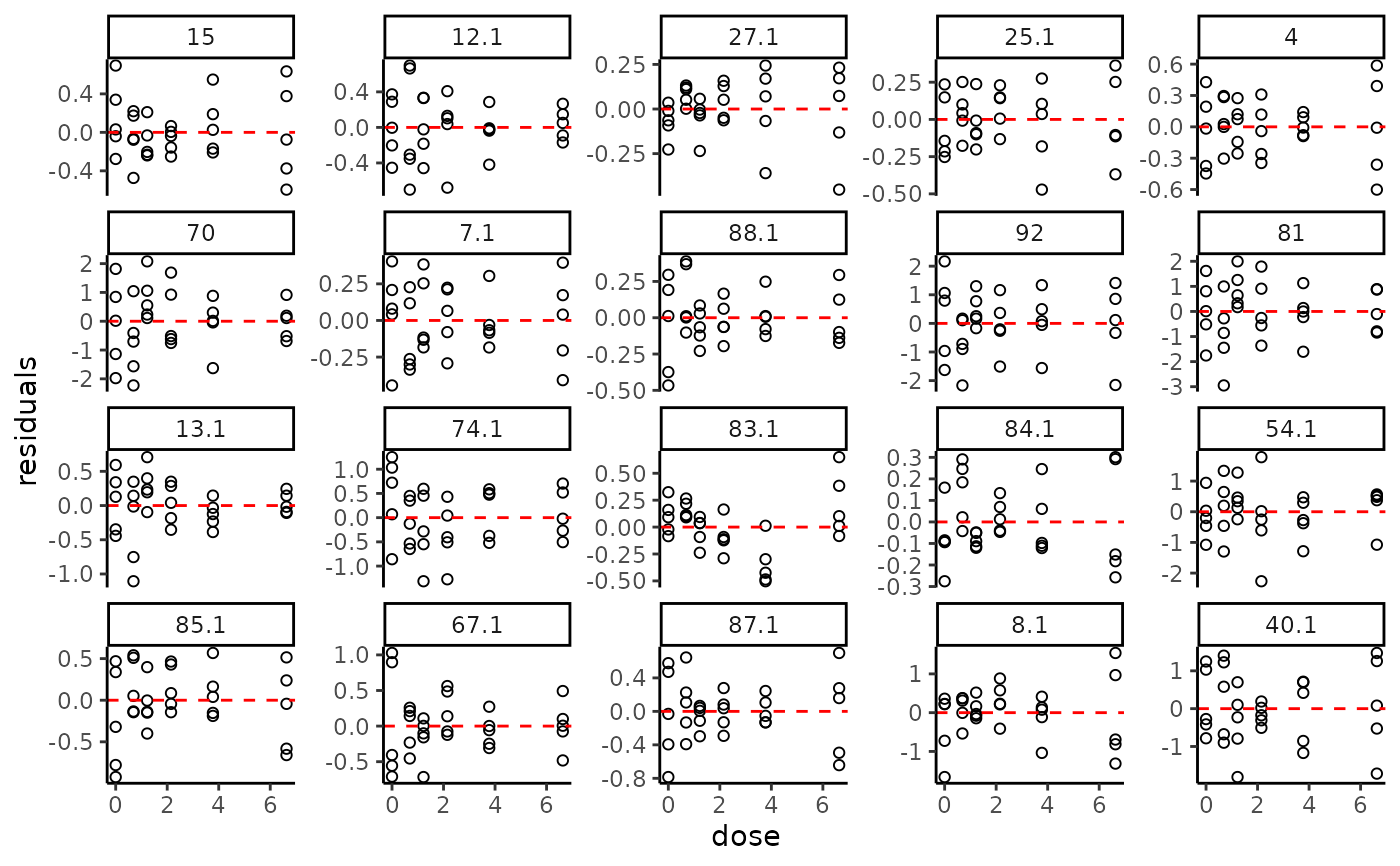
 # Plot of residuals as function of the dose
plot(f, plot.type = "dose_residuals")
#> Warning: Transformation introduced infinite values in continuous x-axis
# Plot of residuals as function of the dose
plot(f, plot.type = "dose_residuals")
#> Warning: Transformation introduced infinite values in continuous x-axis
 # Same plot of residuals without log transformation of the doses
plot(f, plot.type = "dose_residuals", dose_log_transfo = FALSE)
# Same plot of residuals without log transformation of the doses
plot(f, plot.type = "dose_residuals", dose_log_transfo = FALSE)
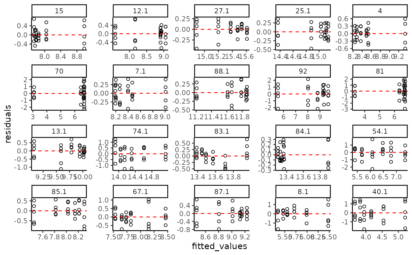
 # plot of residuals as function of the fitted value
plot(f, plot.type = "fitted_residuals")
# plot of residuals as function of the fitted value
plot(f, plot.type = "fitted_residuals")
 # (2) an example on a microarray data set (a subsample of a greater data set)
#
datafilename <- system.file("extdata", "transcripto_sample.txt", package = "DRomics")
(o <- microarraydata(datafilename, check = TRUE, norm.method = "cyclicloess"))
#> Just wait, the normalization using cyclicloess may take a few minutes.
#> Elements of the experimental design in order to check the coding of the data:
#> Tested doses and number of replicates for each dose:
#>
#> 0 0.69 1.223 2.148 3.774 6.631
#> 5 5 5 5 5 5
#> Number of items: 1000
#> Identifiers of the first 20 items:
#> [1] "1" "2" "3" "4" "5.1" "5.2" "6.1" "6.2" "7.1" "7.2"
#> [11] "8.1" "8.2" "9.1" "9.2" "10.1" "10.2" "11.1" "11.2" "12.1" "12.2"
#> Data were normalized between arrays using the following method: cyclicloess
(s_quad <- itemselect(o, select.method = "quadratic", FDR = 0.05))
#> Removing intercept from test coefficients
#> Number of selected items using a quadratic trend test with an FDR of 0.05: 318
#> Identifiers of the first 20 most responsive items:
#> [1] "384.2" "383.1" "383.2" "384.1" "301.1" "363.1" "300.2" "364.2" "364.1"
#> [10] "363.2" "301.2" "300.1" "351.1" "350.2" "239.1" "240.1" "240.2" "370"
#> [19] "15" "350.1"
(f <- drcfit(s_quad, progressbar = TRUE))
#> The fitting may be long if the number of selected items is high.
#>
|
| | 0%
|
| | 1%
|
|= | 1%
|
|= | 2%
|
|== | 2%
|
|== | 3%
|
|=== | 4%
|
|=== | 5%
|
|==== | 5%
|
|==== | 6%
|
|===== | 7%
|
|===== | 8%
|
|====== | 8%
|
|====== | 9%
|
|======= | 9%
|
|======= | 10%
|
|======= | 11%
|
|======== | 11%
|
|======== | 12%
|
|========= | 12%
|
|========= | 13%
|
|========= | 14%
|
|========== | 14%
|
|========== | 15%
|
|=========== | 15%
|
|=========== | 16%
|
|============ | 17%
|
|============ | 18%
|
|============= | 18%
|
|============= | 19%
|
|============== | 19%
|
|============== | 20%
|
|=============== | 21%
|
|=============== | 22%
|
|================ | 22%
|
|================ | 23%
|
|================= | 24%
|
|================= | 25%
|
|================== | 25%
|
|================== | 26%
|
|=================== | 27%
|
|=================== | 28%
|
|==================== | 28%
|
|==================== | 29%
|
|===================== | 30%
|
|===================== | 31%
|
|====================== | 31%
|
|====================== | 32%
|
|======================= | 32%
|
|======================= | 33%
|
|======================== | 34%
|
|======================== | 35%
|
|========================= | 35%
|
|========================= | 36%
|
|========================== | 36%
|
|========================== | 37%
|
|========================== | 38%
|
|=========================== | 38%
|
|=========================== | 39%
|
|============================ | 39%
|
|============================ | 40%
|
|============================ | 41%
|
|============================= | 41%
|
|============================= | 42%
|
|============================== | 42%
|
|============================== | 43%
|
|=============================== | 44%
|
|=============================== | 45%
|
|================================ | 45%
|
|================================ | 46%
|
|================================= | 47%
|
|================================= | 48%
|
|================================== | 48%
|
|================================== | 49%
|
|=================================== | 49%
|
|=================================== | 50%
|
|=================================== | 51%
|
|==================================== | 51%
|
|==================================== | 52%
|
|===================================== | 52%
|
|===================================== | 53%
|
|====================================== | 54%
|
|====================================== | 55%
|
|======================================= | 55%
|
|======================================= | 56%
|
|======================================== | 57%
|
|======================================== | 58%
|
|========================================= | 58%
|
|========================================= | 59%
|
|========================================== | 59%
|
|========================================== | 60%
|
|========================================== | 61%
|
|=========================================== | 61%
|
|=========================================== | 62%
|
|============================================ | 62%
|
|============================================ | 63%
|
|============================================ | 64%
|
|============================================= | 64%
|
|============================================= | 65%
|
|============================================== | 65%
|
|============================================== | 66%
|
|=============================================== | 67%
|
|=============================================== | 68%
|
|================================================ | 68%
|
|================================================ | 69%
|
|================================================= | 69%
|
|================================================= | 70%
|
|================================================== | 71%
|
|================================================== | 72%
|
|=================================================== | 72%
|
|=================================================== | 73%
|
|==================================================== | 74%
|
|==================================================== | 75%
|
|===================================================== | 75%
|
|===================================================== | 76%
|
|====================================================== | 77%
|
|====================================================== | 78%
|
|======================================================= | 78%
|
|======================================================= | 79%
|
|======================================================== | 80%
|
|======================================================== | 81%
|
|========================================================= | 81%
|
|========================================================= | 82%
|
|========================================================== | 82%
|
|========================================================== | 83%
|
|=========================================================== | 84%
|
|=========================================================== | 85%
|
|============================================================ | 85%
|
|============================================================ | 86%
|
|============================================================= | 86%
|
|============================================================= | 87%
|
|============================================================= | 88%
|
|============================================================== | 88%
|
|============================================================== | 89%
|
|=============================================================== | 89%
|
|=============================================================== | 90%
|
|=============================================================== | 91%
|
|================================================================ | 91%
|
|================================================================ | 92%
|
|================================================================= | 92%
|
|================================================================= | 93%
|
|================================================================== | 94%
|
|================================================================== | 95%
|
|=================================================================== | 95%
|
|=================================================================== | 96%
|
|==================================================================== | 97%
|
|==================================================================== | 98%
|
|===================================================================== | 98%
|
|===================================================================== | 99%
|
|======================================================================| 99%
|
|======================================================================| 100%
#> Results of the fitting using the AICc to select the best fit model
#> 60 dose-response curves out of 318 previously selected were removed
#> because no model could be fitted reliably.
#> Distribution of the chosen models among the 258 fitted dose-response curves:
#>
#> Hill linear exponential Gauss-probit
#> 2 85 64 89
#> log-Gauss-probit
#> 18
#> Distribution of the trends (curve shapes) among the 258 fitted dose-response curves:
#>
#> U bell dec inc
#> 55 52 58 93
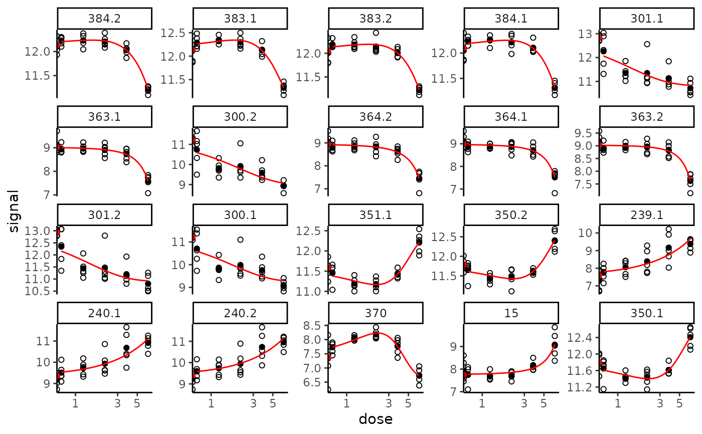
# Default plot
plot(f)
#> Warning: Transformation introduced infinite values in continuous x-axis
#> Warning: Transformation introduced infinite values in continuous x-axis
#> Warning: Transformation introduced infinite values in continuous x-axis
# (2) an example on a microarray data set (a subsample of a greater data set)
#
datafilename <- system.file("extdata", "transcripto_sample.txt", package = "DRomics")
(o <- microarraydata(datafilename, check = TRUE, norm.method = "cyclicloess"))
#> Just wait, the normalization using cyclicloess may take a few minutes.
#> Elements of the experimental design in order to check the coding of the data:
#> Tested doses and number of replicates for each dose:
#>
#> 0 0.69 1.223 2.148 3.774 6.631
#> 5 5 5 5 5 5
#> Number of items: 1000
#> Identifiers of the first 20 items:
#> [1] "1" "2" "3" "4" "5.1" "5.2" "6.1" "6.2" "7.1" "7.2"
#> [11] "8.1" "8.2" "9.1" "9.2" "10.1" "10.2" "11.1" "11.2" "12.1" "12.2"
#> Data were normalized between arrays using the following method: cyclicloess
(s_quad <- itemselect(o, select.method = "quadratic", FDR = 0.05))
#> Removing intercept from test coefficients
#> Number of selected items using a quadratic trend test with an FDR of 0.05: 318
#> Identifiers of the first 20 most responsive items:
#> [1] "384.2" "383.1" "383.2" "384.1" "301.1" "363.1" "300.2" "364.2" "364.1"
#> [10] "363.2" "301.2" "300.1" "351.1" "350.2" "239.1" "240.1" "240.2" "370"
#> [19] "15" "350.1"
(f <- drcfit(s_quad, progressbar = TRUE))
#> The fitting may be long if the number of selected items is high.
#>
|
| | 0%
|
| | 1%
|
|= | 1%
|
|= | 2%
|
|== | 2%
|
|== | 3%
|
|=== | 4%
|
|=== | 5%
|
|==== | 5%
|
|==== | 6%
|
|===== | 7%
|
|===== | 8%
|
|====== | 8%
|
|====== | 9%
|
|======= | 9%
|
|======= | 10%
|
|======= | 11%
|
|======== | 11%
|
|======== | 12%
|
|========= | 12%
|
|========= | 13%
|
|========= | 14%
|
|========== | 14%
|
|========== | 15%
|
|=========== | 15%
|
|=========== | 16%
|
|============ | 17%
|
|============ | 18%
|
|============= | 18%
|
|============= | 19%
|
|============== | 19%
|
|============== | 20%
|
|=============== | 21%
|
|=============== | 22%
|
|================ | 22%
|
|================ | 23%
|
|================= | 24%
|
|================= | 25%
|
|================== | 25%
|
|================== | 26%
|
|=================== | 27%
|
|=================== | 28%
|
|==================== | 28%
|
|==================== | 29%
|
|===================== | 30%
|
|===================== | 31%
|
|====================== | 31%
|
|====================== | 32%
|
|======================= | 32%
|
|======================= | 33%
|
|======================== | 34%
|
|======================== | 35%
|
|========================= | 35%
|
|========================= | 36%
|
|========================== | 36%
|
|========================== | 37%
|
|========================== | 38%
|
|=========================== | 38%
|
|=========================== | 39%
|
|============================ | 39%
|
|============================ | 40%
|
|============================ | 41%
|
|============================= | 41%
|
|============================= | 42%
|
|============================== | 42%
|
|============================== | 43%
|
|=============================== | 44%
|
|=============================== | 45%
|
|================================ | 45%
|
|================================ | 46%
|
|================================= | 47%
|
|================================= | 48%
|
|================================== | 48%
|
|================================== | 49%
|
|=================================== | 49%
|
|=================================== | 50%
|
|=================================== | 51%
|
|==================================== | 51%
|
|==================================== | 52%
|
|===================================== | 52%
|
|===================================== | 53%
|
|====================================== | 54%
|
|====================================== | 55%
|
|======================================= | 55%
|
|======================================= | 56%
|
|======================================== | 57%
|
|======================================== | 58%
|
|========================================= | 58%
|
|========================================= | 59%
|
|========================================== | 59%
|
|========================================== | 60%
|
|========================================== | 61%
|
|=========================================== | 61%
|
|=========================================== | 62%
|
|============================================ | 62%
|
|============================================ | 63%
|
|============================================ | 64%
|
|============================================= | 64%
|
|============================================= | 65%
|
|============================================== | 65%
|
|============================================== | 66%
|
|=============================================== | 67%
|
|=============================================== | 68%
|
|================================================ | 68%
|
|================================================ | 69%
|
|================================================= | 69%
|
|================================================= | 70%
|
|================================================== | 71%
|
|================================================== | 72%
|
|=================================================== | 72%
|
|=================================================== | 73%
|
|==================================================== | 74%
|
|==================================================== | 75%
|
|===================================================== | 75%
|
|===================================================== | 76%
|
|====================================================== | 77%
|
|====================================================== | 78%
|
|======================================================= | 78%
|
|======================================================= | 79%
|
|======================================================== | 80%
|
|======================================================== | 81%
|
|========================================================= | 81%
|
|========================================================= | 82%
|
|========================================================== | 82%
|
|========================================================== | 83%
|
|=========================================================== | 84%
|
|=========================================================== | 85%
|
|============================================================ | 85%
|
|============================================================ | 86%
|
|============================================================= | 86%
|
|============================================================= | 87%
|
|============================================================= | 88%
|
|============================================================== | 88%
|
|============================================================== | 89%
|
|=============================================================== | 89%
|
|=============================================================== | 90%
|
|=============================================================== | 91%
|
|================================================================ | 91%
|
|================================================================ | 92%
|
|================================================================= | 92%
|
|================================================================= | 93%
|
|================================================================== | 94%
|
|================================================================== | 95%
|
|=================================================================== | 95%
|
|=================================================================== | 96%
|
|==================================================================== | 97%
|
|==================================================================== | 98%
|
|===================================================================== | 98%
|
|===================================================================== | 99%
|
|======================================================================| 99%
|
|======================================================================| 100%
#> Results of the fitting using the AICc to select the best fit model
#> 60 dose-response curves out of 318 previously selected were removed
#> because no model could be fitted reliably.
#> Distribution of the chosen models among the 258 fitted dose-response curves:
#>
#> Hill linear exponential Gauss-probit
#> 2 85 64 89
#> log-Gauss-probit
#> 18
#> Distribution of the trends (curve shapes) among the 258 fitted dose-response curves:
#>
#> U bell dec inc
#> 55 52 58 93
# Default plot
plot(f)
#> Warning: Transformation introduced infinite values in continuous x-axis
#> Warning: Transformation introduced infinite values in continuous x-axis
#> Warning: Transformation introduced infinite values in continuous x-axis
 # save all plots to pdf using plotfit2pdf()
plotfit2pdf(f, path2figs = tempdir())
#>
#> Figures are stored in /tmp/RtmpxHwo3c.
#> Warning: Transformation introduced infinite values in continuous x-axis
#> Warning: Transformation introduced infinite values in continuous x-axis
#> Warning: Transformation introduced infinite values in continuous x-axis
#> Warning: Transformation introduced infinite values in continuous x-axis
#> Warning: Transformation introduced infinite values in continuous x-axis
#> Warning: Transformation introduced infinite values in continuous x-axis
#> Warning: Transformation introduced infinite values in continuous x-axis
#> Warning: Transformation introduced infinite values in continuous x-axis
#> Warning: Transformation introduced infinite values in continuous x-axis
#> Warning: Transformation introduced infinite values in continuous x-axis
#> Warning: Transformation introduced infinite values in continuous x-axis
#> Warning: Transformation introduced infinite values in continuous x-axis
#> Warning: Transformation introduced infinite values in continuous x-axis
#> Warning: Transformation introduced infinite values in continuous x-axis
#> Warning: Transformation introduced infinite values in continuous x-axis
#> Warning: Transformation introduced infinite values in continuous x-axis
#> Warning: Transformation introduced infinite values in continuous x-axis
#> Warning: Transformation introduced infinite values in continuous x-axis
#> Warning: Transformation introduced infinite values in continuous x-axis
#> Warning: Transformation introduced infinite values in continuous x-axis
#> Warning: Transformation introduced infinite values in continuous x-axis
#> Warning: Transformation introduced infinite values in continuous x-axis
#> Warning: Transformation introduced infinite values in continuous x-axis
#> Warning: Transformation introduced infinite values in continuous x-axis
#> Warning: Transformation introduced infinite values in continuous x-axis
#> Warning: Transformation introduced infinite values in continuous x-axis
#> Warning: Transformation introduced infinite values in continuous x-axis
#> Warning: Transformation introduced infinite values in continuous x-axis
#> Warning: Transformation introduced infinite values in continuous x-axis
#> Warning: Transformation introduced infinite values in continuous x-axis
#> Warning: Transformation introduced infinite values in continuous x-axis
#> Warning: Transformation introduced infinite values in continuous x-axis
#> Warning: Transformation introduced infinite values in continuous x-axis
#> agg_png
#> 2
plotfit2pdf(f, plot.type = "fitted_residuals",
nrowperpage = 9, ncolperpage = 6, path2figs = tempdir())
#>
#> Figures are stored in /tmp/RtmpxHwo3c.
#> agg_png
#> 2
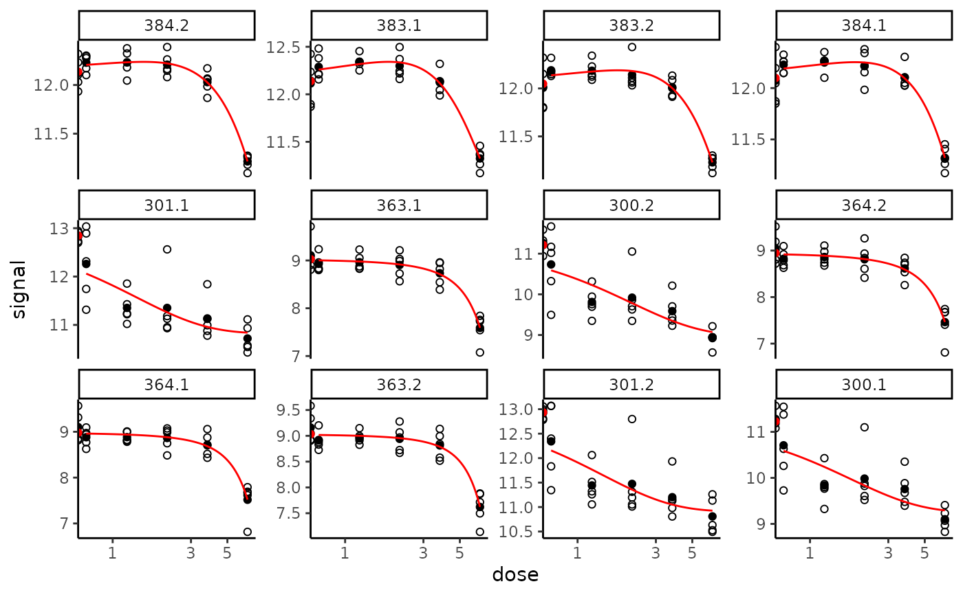
# Plot of the fit of the first 12 most responsive items
plot(f, items = 12)
#> Warning: Transformation introduced infinite values in continuous x-axis
#> Warning: Transformation introduced infinite values in continuous x-axis
#> Warning: Transformation introduced infinite values in continuous x-axis
# save all plots to pdf using plotfit2pdf()
plotfit2pdf(f, path2figs = tempdir())
#>
#> Figures are stored in /tmp/RtmpxHwo3c.
#> Warning: Transformation introduced infinite values in continuous x-axis
#> Warning: Transformation introduced infinite values in continuous x-axis
#> Warning: Transformation introduced infinite values in continuous x-axis
#> Warning: Transformation introduced infinite values in continuous x-axis
#> Warning: Transformation introduced infinite values in continuous x-axis
#> Warning: Transformation introduced infinite values in continuous x-axis
#> Warning: Transformation introduced infinite values in continuous x-axis
#> Warning: Transformation introduced infinite values in continuous x-axis
#> Warning: Transformation introduced infinite values in continuous x-axis
#> Warning: Transformation introduced infinite values in continuous x-axis
#> Warning: Transformation introduced infinite values in continuous x-axis
#> Warning: Transformation introduced infinite values in continuous x-axis
#> Warning: Transformation introduced infinite values in continuous x-axis
#> Warning: Transformation introduced infinite values in continuous x-axis
#> Warning: Transformation introduced infinite values in continuous x-axis
#> Warning: Transformation introduced infinite values in continuous x-axis
#> Warning: Transformation introduced infinite values in continuous x-axis
#> Warning: Transformation introduced infinite values in continuous x-axis
#> Warning: Transformation introduced infinite values in continuous x-axis
#> Warning: Transformation introduced infinite values in continuous x-axis
#> Warning: Transformation introduced infinite values in continuous x-axis
#> Warning: Transformation introduced infinite values in continuous x-axis
#> Warning: Transformation introduced infinite values in continuous x-axis
#> Warning: Transformation introduced infinite values in continuous x-axis
#> Warning: Transformation introduced infinite values in continuous x-axis
#> Warning: Transformation introduced infinite values in continuous x-axis
#> Warning: Transformation introduced infinite values in continuous x-axis
#> Warning: Transformation introduced infinite values in continuous x-axis
#> Warning: Transformation introduced infinite values in continuous x-axis
#> Warning: Transformation introduced infinite values in continuous x-axis
#> Warning: Transformation introduced infinite values in continuous x-axis
#> Warning: Transformation introduced infinite values in continuous x-axis
#> Warning: Transformation introduced infinite values in continuous x-axis
#> agg_png
#> 2
plotfit2pdf(f, plot.type = "fitted_residuals",
nrowperpage = 9, ncolperpage = 6, path2figs = tempdir())
#>
#> Figures are stored in /tmp/RtmpxHwo3c.
#> agg_png
#> 2
# Plot of the fit of the first 12 most responsive items
plot(f, items = 12)
#> Warning: Transformation introduced infinite values in continuous x-axis
#> Warning: Transformation introduced infinite values in continuous x-axis
#> Warning: Transformation introduced infinite values in continuous x-axis
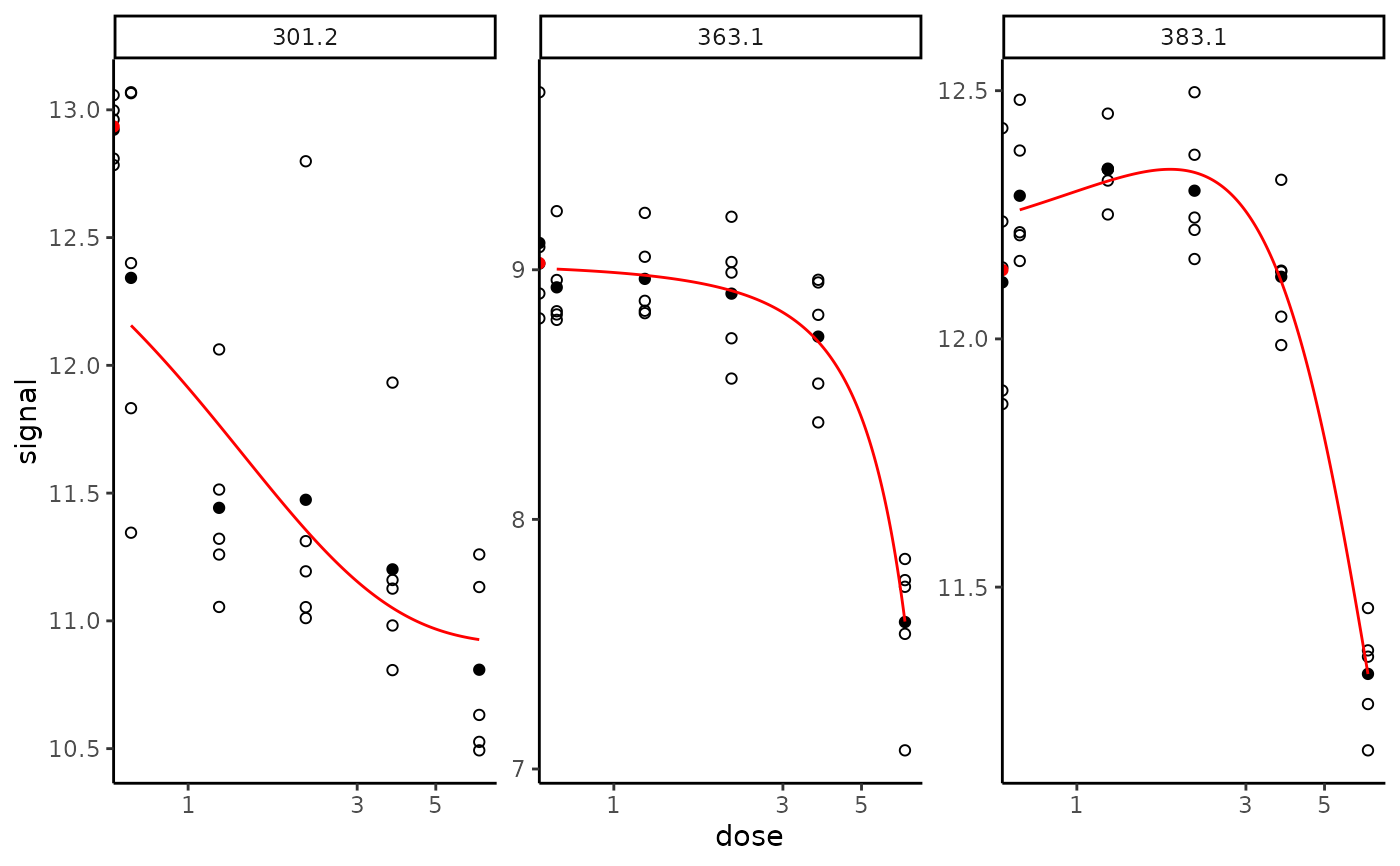
 # Plot of the chosen items in the chosen order
plot(f, items = c("301.2", "363.1", "383.1"))
#> Warning: Transformation introduced infinite values in continuous x-axis
#> Warning: Transformation introduced infinite values in continuous x-axis
#> Warning: Transformation introduced infinite values in continuous x-axis
# Plot of the chosen items in the chosen order
plot(f, items = c("301.2", "363.1", "383.1"))
#> Warning: Transformation introduced infinite values in continuous x-axis
#> Warning: Transformation introduced infinite values in continuous x-axis
#> Warning: Transformation introduced infinite values in continuous x-axis
 # Look at the table of results for successful fits
head(f$fitres)
#> id irow adjpvalue model nbpar b c d
#> 1 384.2 727 2.519524e-07 Gauss-probit 4 8.39021007 6.160174 6.160174
#> 2 383.1 724 6.558388e-07 Gauss-probit 4 3.81611448 10.480252 10.480252
#> 3 383.2 725 8.234946e-07 Gauss-probit 4 6.27817663 8.505693 8.505693
#> 4 384.1 726 2.804671e-06 Gauss-probit 4 8.59581518 5.684089 5.684089
#> 5 301.1 569 6.932747e-06 exponential 3 2.02444957 NA 12.846110
#> 6 363.1 686 7.084800e-06 exponential 3 -0.06029708 NA 9.026630
#> e f SDres typology trend y0 yatdosemax
#> 1 1.538640 6.077561 0.1126233 GP.bell bell 12.13639 11.215361
#> 2 1.833579 1.861385 0.1411563 GP.bell bell 12.13871 11.324854
#> 3 1.751051 3.683404 0.1335847 GP.bell bell 12.04858 11.228734
#> 4 1.874867 6.568752 0.1379656 GP.bell bell 12.09844 11.320509
#> 5 -1.404111 NA 0.4905313 E.dec.convex dec 12.84611 10.839662
#> 6 2.064800 NA 0.2526946 E.dec.concave dec 9.02663 7.590655
#> yrange maxychange xextrem yextrem
#> 1 1.0223735 0.9210335 1.538640 12.23774
#> 2 1.0167830 0.8138568 1.833579 12.34164
#> 3 0.9603629 0.8198451 1.751051 12.18910
#> 4 0.9323327 0.7779265 1.874867 12.25284
#> 5 2.0064474 2.0064474 NA NA
#> 6 1.4359752 1.4359752 NA NA
# Look at the table of results for unsuccessful fits
head(f$unfitres)
#> id irow adjpvalue cause
#> 25 368.1 696 5.865601e-05 trend.in.residuals
#> 38 367.1 694 2.748644e-04 trend.in.residuals
#> 51 360.2 681 3.964071e-04 trend.in.residuals
#> 57 162.2 305 4.818750e-04 trend.in.residuals
#> 59 161.1 302 5.387711e-04 trend.in.residuals
#> 60 275.1 519 5.387711e-04 trend.in.residuals
# count the number of unsuccessful fits for each cause
table(f$unfitres$cause)
#>
#> constant.model trend.in.residuals
#> 30 30
# (3) Comparison of parallel and non paralell implementations on a larger selection of items
#
if(!requireNamespace("parallel", quietly = TRUE)) {
if(parallel::detectCores() > 1) {
s_quad <- itemselect(o, select.method = "quadratic", FDR = 0.05)
system.time(f1 <- drcfit(s_quad, progressbar = TRUE))
system.time(f2 <- drcfit(s_quad, progressbar = FALSE, parallel = "snow", ncpus = 2))
}}
# }
# Look at the table of results for successful fits
head(f$fitres)
#> id irow adjpvalue model nbpar b c d
#> 1 384.2 727 2.519524e-07 Gauss-probit 4 8.39021007 6.160174 6.160174
#> 2 383.1 724 6.558388e-07 Gauss-probit 4 3.81611448 10.480252 10.480252
#> 3 383.2 725 8.234946e-07 Gauss-probit 4 6.27817663 8.505693 8.505693
#> 4 384.1 726 2.804671e-06 Gauss-probit 4 8.59581518 5.684089 5.684089
#> 5 301.1 569 6.932747e-06 exponential 3 2.02444957 NA 12.846110
#> 6 363.1 686 7.084800e-06 exponential 3 -0.06029708 NA 9.026630
#> e f SDres typology trend y0 yatdosemax
#> 1 1.538640 6.077561 0.1126233 GP.bell bell 12.13639 11.215361
#> 2 1.833579 1.861385 0.1411563 GP.bell bell 12.13871 11.324854
#> 3 1.751051 3.683404 0.1335847 GP.bell bell 12.04858 11.228734
#> 4 1.874867 6.568752 0.1379656 GP.bell bell 12.09844 11.320509
#> 5 -1.404111 NA 0.4905313 E.dec.convex dec 12.84611 10.839662
#> 6 2.064800 NA 0.2526946 E.dec.concave dec 9.02663 7.590655
#> yrange maxychange xextrem yextrem
#> 1 1.0223735 0.9210335 1.538640 12.23774
#> 2 1.0167830 0.8138568 1.833579 12.34164
#> 3 0.9603629 0.8198451 1.751051 12.18910
#> 4 0.9323327 0.7779265 1.874867 12.25284
#> 5 2.0064474 2.0064474 NA NA
#> 6 1.4359752 1.4359752 NA NA
# Look at the table of results for unsuccessful fits
head(f$unfitres)
#> id irow adjpvalue cause
#> 25 368.1 696 5.865601e-05 trend.in.residuals
#> 38 367.1 694 2.748644e-04 trend.in.residuals
#> 51 360.2 681 3.964071e-04 trend.in.residuals
#> 57 162.2 305 4.818750e-04 trend.in.residuals
#> 59 161.1 302 5.387711e-04 trend.in.residuals
#> 60 275.1 519 5.387711e-04 trend.in.residuals
# count the number of unsuccessful fits for each cause
table(f$unfitres$cause)
#>
#> constant.model trend.in.residuals
#> 30 30
# (3) Comparison of parallel and non paralell implementations on a larger selection of items
#
if(!requireNamespace("parallel", quietly = TRUE)) {
if(parallel::detectCores() > 1) {
s_quad <- itemselect(o, select.method = "quadratic", FDR = 0.05)
system.time(f1 <- drcfit(s_quad, progressbar = TRUE))
system.time(f2 <- drcfit(s_quad, progressbar = FALSE, parallel = "snow", ncpus = 2))
}}
# }