Import, check and normalization of single-channel microarray data

Single-channel microarray data in log2 are imported from a .txt file (internally imported using the function read.table), checked or from a R object of class data.frame (see the description of argument file for the required format of data)and normalized (between arrays normalization). omicdata is a deprecated version of microarraydata.

Usage

microarraydata(file, backgrounddose, check = TRUE, 
  norm.method = c("cyclicloess", "quantile", "scale", "none"))
  
omicdata(file, backgrounddose, check = TRUE, 
  norm.method = c("cyclicloess", "quantile", "scale", "none"))

# S3 method for microarraydata
print(x, ...)
# S3 method for microarraydata
plot(x, range4boxplot = 0, ...)

Arguments

file: The name of the .txt file (e.g. "mydata.txt") containing one row per item, with the first column corresponding to the identifier of each item, and the other columns giving the responses of the item for each replicate at each dose or concentration. In the first line, after a name for the identifier column, we must have the tested doses or concentrations in a numeric format for the corresponding replicate (for example, if there are triplicates for each treatment, the first line could be "item", 0, 0, 0, 0.1, 0.1, 0.1, etc.). This file is imported within the function using the function read.table with its default field separator (sep argument) and its default decimal separator (dec argument at "."). Alternatively an R object of class data.frame can be directly given in input, corresponding to the output of read.table(file, header = FALSE) on a file described as above.
backgrounddose: This argument must be used when there is no dose at zero in the data, to prevent the calculation of the BMD by extrapolation. All doses below or equal to the value given in backgrounddose will be fixed at 0, so as to be considered at the background level of exposition.
check: If TRUE the format of the input file is checked.
norm.method: If "none" no normalization is performed, else a normalization is performed using the function normalizeBetweenArrays of the limma package using the specified method.
x: An object of class "microarraydata".
range4boxplot: An argument passed to boxplot(), fixed by default at 0 to prevent the producing of very large plot files due to many outliers. Can be put at 1.5 to obtain more classical boxplots.
...: further arguments passed to print or plot functions.

Details

This function imports the data, checks their format (see the description of argument file for the required format of data) and gives in the print information that should help the user to check that the coding of data is correct : the tested doses (or concentrations) the number of replicates for each dose, the number of items, the identifiers of the first 20 items. If the argument norm.method is not "none", data are normalized using the function normalizeBetweenArrays of the limma package using the specified method : "cyclicloess" (default choice), "quantile" or "scale".

Value

microarraydata returns an object of class "microarraydata", a list with 9 components:

data: the numeric matrix of normalized responses of each item in each replicate (one line per item, one column per replicate)
dose: the numeric vector of the tested doses or concentrations corresponding to each column of data
item: the character vector of the identifiers of the items, corresponding to each line of data
design: a table with the experimental design (tested doses and number of replicates for each dose) for control by the user
data.mean: the numeric matrix of mean responses of each item per dose (mean of the corresponding replicates) (one line per item, one column per unique value of the dose
data.sd: the numeric matrix of standard deviations of the response of each item per dose (sd of the corresponding replicates, NA if no replicate) (one line per item, one column per unique value of the dose)
norm.method: The normalization method specified in input
data.beforenorm: the numeric matrix of responses of each item in each replicate (one line per item, one column per replicate) before normalization
containsNA: always at FALSE as microarray data are not allowed to contain NA values

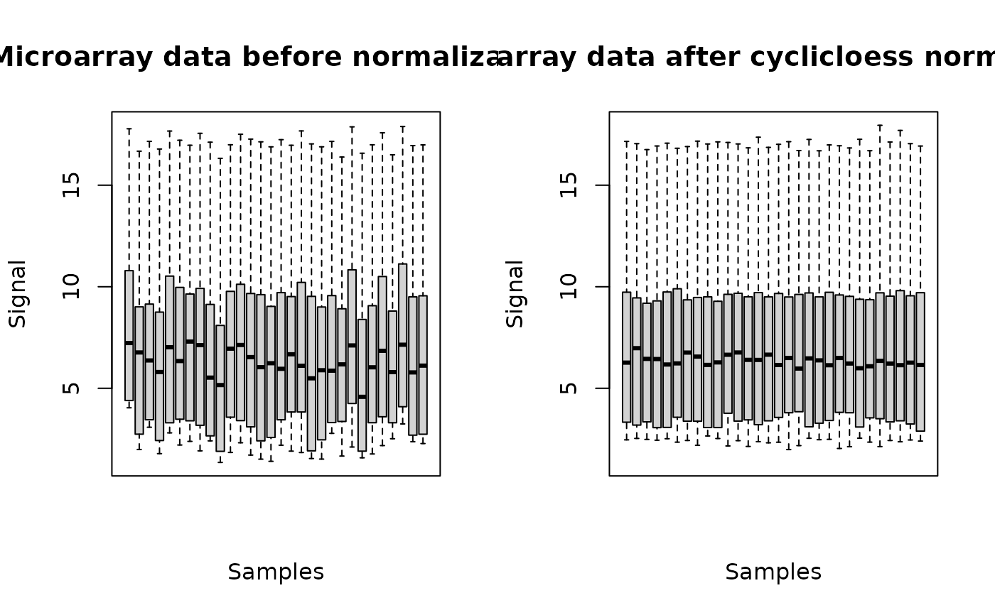
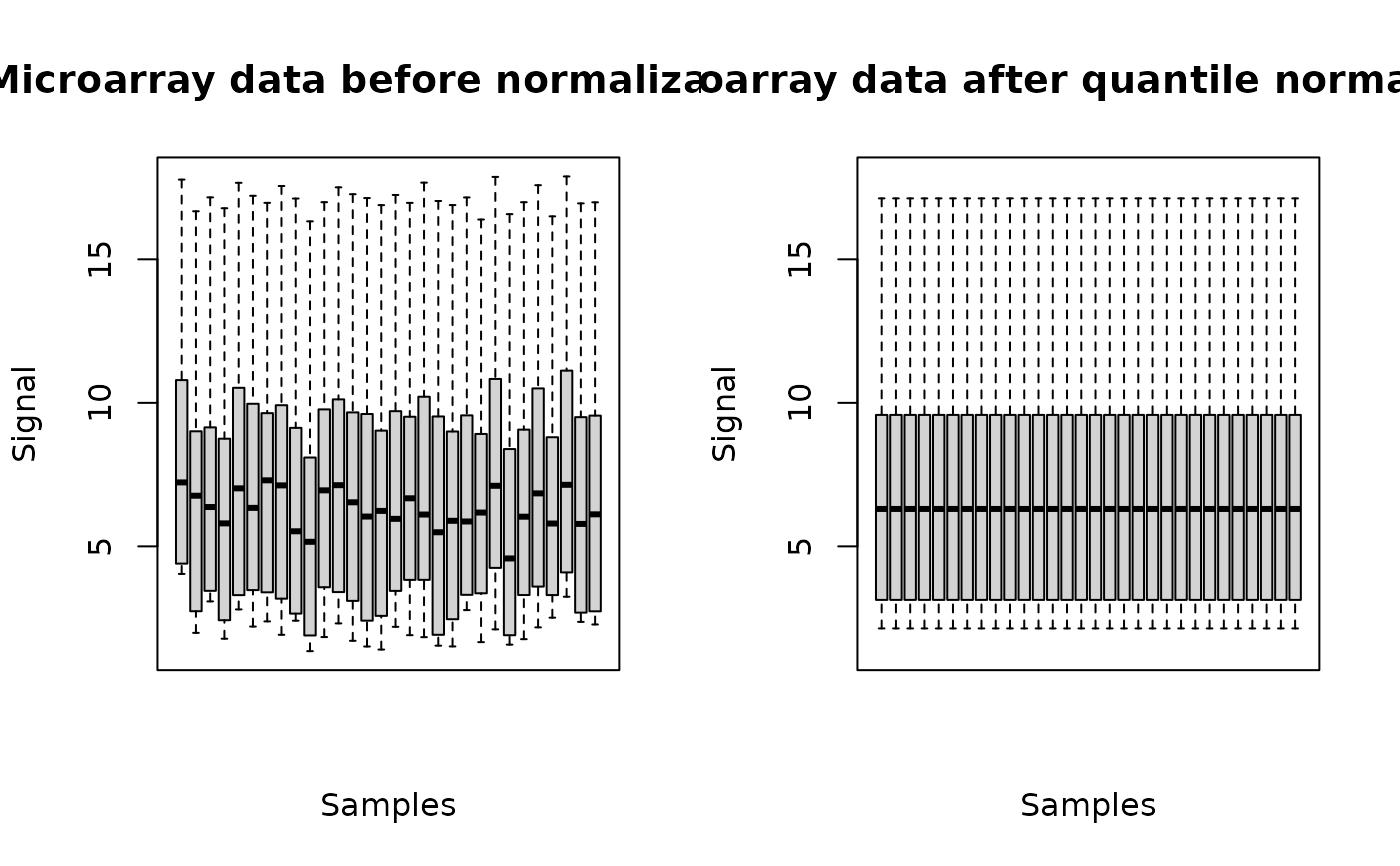
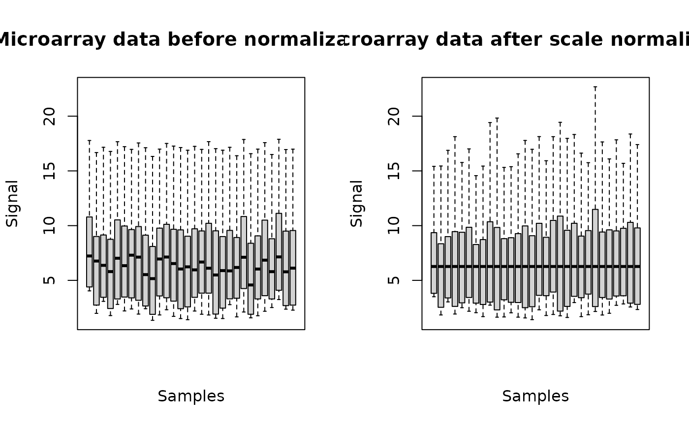
The print of a microarraydata object gives the tested doses (or concentrations) and number of replicates for each dose, the number of items, the identifiers of the first 20 items (for check of good coding of data) and the normalization method. The plot of a microarraydata object shows the data distribution for each dose or concentration and replicate before and after normalization.

References

Ritchie ME, Phipson B, Wu D, Hu Y, Law CW, Shi W, and Smyth, GK (2015), limma powers differential expression analyses for RNA-sequencing and microarray studies. Nucleic Acids Research 43, e47.

Author

Marie-Laure Delignette-Muller

Examples

# (1) import, check and normalization of microarray data 
# (an example on a subsample of a greater data set published in Larras et al. 2018
# Transcriptomic effect of triclosan in the chlorophyte Scenedesmus vacuolatus)
datafilename <- system.file("extdata", "transcripto_very_small_sample.txt", 
  package="DRomics")
o <- microarraydata(datafilename, check = TRUE, norm.method = "cyclicloess")
#> Just wait, the normalization using cyclicloess may take a few minutes.
print(o)
#> Elements of the experimental design in order to check the coding of the data:
#> Tested doses and number of replicates for each dose:
#> 
#>     0  0.69 1.223 2.148 3.774 6.631 
#>     5     5     5     5     5     5 
#> Number of items: 100 
#> Identifiers of the first 20 items:
#>  [1] "1"    "2"    "3"    "4"    "5.1"  "6.1"  "7.1"  "8.1"  "9.1"  "10.1"
#> [11] "11.1" "12.1" "13.1" "14.1" "15"   "16.1" "17.1" "18.1" "19.1" "20.1"
#> Data were normalized between arrays using the following method: cyclicloess 
plot(o)

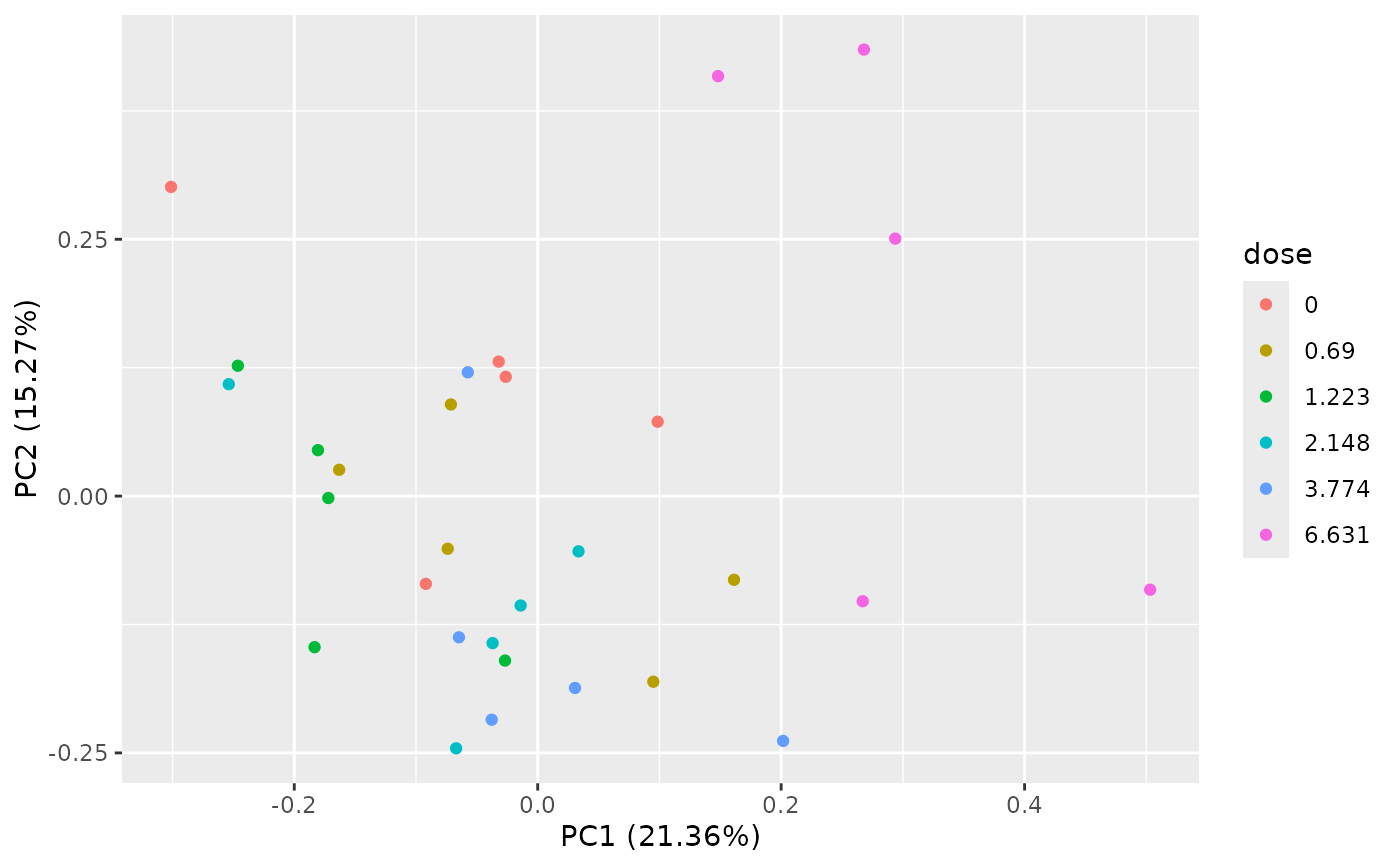
PCAdataplot(o)

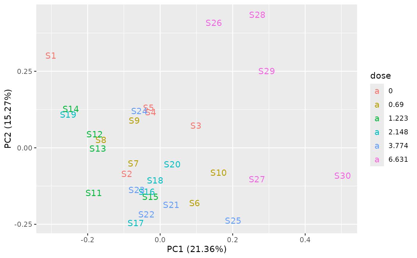
PCAdataplot(o, label = TRUE)



# If you want to use your own data set just replace datafilename, 
# the first argument of microarraydata(), 
# by the name of your data file (e.g. "mydata.txt")
# 
# You should take care that the field separator of this data file is one
# of the default field separators recognised by the read.table() function
# when it is used with its default field separator (sep argument)
# Tabs are recommended.

# \donttest{

# (2) normalization with other methods
(o.2 <- microarraydata(datafilename, check = TRUE, norm.method = "quantile"))
#> Elements of the experimental design in order to check the coding of the data:
#> Tested doses and number of replicates for each dose:
#> 
#>     0  0.69 1.223 2.148 3.774 6.631 
#>     5     5     5     5     5     5 
#> Number of items: 100 
#> Identifiers of the first 20 items:
#>  [1] "1"    "2"    "3"    "4"    "5.1"  "6.1"  "7.1"  "8.1"  "9.1"  "10.1"
#> [11] "11.1" "12.1" "13.1" "14.1" "15"   "16.1" "17.1" "18.1" "19.1" "20.1"
#> Data were normalized between arrays using the following method: quantile 
plot(o.2)

(o.3 <- microarraydata(datafilename, check = TRUE, norm.method = "scale"))
#> Elements of the experimental design in order to check the coding of the data:
#> Tested doses and number of replicates for each dose:
#> 
#>     0  0.69 1.223 2.148 3.774 6.631 
#>     5     5     5     5     5     5 
#> Number of items: 100 
#> Identifiers of the first 20 items:
#>  [1] "1"    "2"    "3"    "4"    "5.1"  "6.1"  "7.1"  "8.1"  "9.1"  "10.1"
#> [11] "11.1" "12.1" "13.1" "14.1" "15"   "16.1" "17.1" "18.1" "19.1" "20.1"
#> Data were normalized between arrays using the following method: scale 
plot(o.3)


# }