Plot of a summary of BMD values per group of items
sensitivityplot.RdPlot of a summary of BMD values per group of items (with groups defined for example from biological annotation), with groups ordered by values of the chosen summary (as an ECDF plot) or ordered as they are in the definition of the factor coding for them, with points sized by the numbers of items per group.
Arguments
- extendedres
the dataframe of results provided by bmdcalc (res) or a subset of this data frame (selected lines). This dataframe can be extended with additional columns coming for example from the annotation of items, and some lines can be replicated if their corresponding item has more than one annotation. This extended dataframe must at least contain the column giving the chosen BMD values on which to compute the sensitivity (column
BMD.zSDorBMD.xfold).- BMDtype
The type of BMD used,
"zSD"(default choice) or"xfold".- group
the name of the column of extendedres coding for the groups on which we want to estimate a global sensitivity. If
ECDF_plotis FALSE, this column should be a factor ordered as you want the groups to appear in the plot from bottom up.- ECDF_plot
if TRUE (default choice) groups appear ordered by values of the BMD summary value from the bottom up, else they are ordered as their corresponding levels in the factor given in
group. Ifcolorbyis given,ECDF_plotis fixed to FALSE.- colorby
optional argument naming the column of
extendedrescoding for an additional level of grouping that will be materialized by the color. If not missing,ECDF_plotis fixed to FALSE.- BMDsummary
The type of summary used for sensitivity plot,
"first.quartile"(default choice) for the plot of first quartiles of BMD values per group,"median"for the plot of medians of BMD values per group and"median.and.IQR"for the plot of medians with an interval corresponding to the inter-quartile range (IQR).- BMD_log_transfo
If TRUE, default choice, a log transformation of the BMD is used in the plot.
- line.size
Width of the lines.
- line.alpha
Transparency of the lines.
- point.alpha
Transparency of the points.
Details
The chosen summary is calculated on the BMD values for each group (groups can be for example defined as pathways from biological annotation of items) and plotted as an ECDF plot (ordered by the BMD summary) or in the order of the levels of the factor defining the groups from bottom to up. In this plot each point is sized according to the number of items in the corresponding group. Optionally a different levels (e.g. different molecular levels in a multi-omics approach) can be coded by different colors.
See also
See ecdfquantileplot.
Examples
# (1) An example from data published by Larras et al. 2020
# in Journal of Hazardous Materials
# https://doi.org/10.1016/j.jhazmat.2020.122727
# a dataframe with metabolomic results (output $res of bmdcalc() or bmdboot() functions)
resfilename <- system.file("extdata", "triclosanSVmetabres.txt", package="DRomics")
res <- read.table(resfilename, header = TRUE, stringsAsFactors = TRUE)
str(res)
#> 'data.frame': 31 obs. of 27 variables:
#> $ id : Factor w/ 31 levels "NAP47_51","NAP_2",..: 2 3 4 5 6 7 8 9 10 11 ...
#> $ irow : int 2 21 28 34 38 47 49 51 53 67 ...
#> $ adjpvalue : num 6.23e-05 1.11e-05 1.03e-05 1.89e-03 4.16e-03 ...
#> $ model : Factor w/ 4 levels "Gauss-probit",..: 2 3 3 2 2 4 2 2 3 3 ...
#> $ nbpar : int 3 2 2 3 3 5 3 3 2 2 ...
#> $ b : num 0.4598 -0.0595 -0.0451 0.6011 0.6721 ...
#> $ c : num NA NA NA NA NA ...
#> $ d : num 5.94 5.39 7.86 6.86 6.21 ...
#> $ e : num -1.648 NA NA -0.321 -0.323 ...
#> $ f : num NA NA NA NA NA ...
#> $ SDres : num 0.126 0.0793 0.052 0.2338 0.2897 ...
#> $ typology : Factor w/ 10 levels "E.dec.concave",..: 2 7 7 2 2 9 2 2 7 7 ...
#> $ trend : Factor w/ 4 levels "U","bell","dec",..: 3 3 3 3 3 1 3 3 3 3 ...
#> $ y0 : num 5.94 5.39 7.86 6.86 6.21 ...
#> $ yrange : num 0.456 0.461 0.35 0.601 0.672 ...
#> $ maxychange : num 0.456 0.461 0.35 0.601 0.672 ...
#> $ xextrem : num NA NA NA NA NA ...
#> $ yextrem : num NA NA NA NA NA ...
#> $ BMD.zSD : num 0.528 1.333 1.154 0.158 0.182 ...
#> $ BMR.zSD : num 5.82 5.31 7.81 6.62 5.92 ...
#> $ BMD.xfold : num NA NA NA NA 0.832 ...
#> $ BMR.xfold : num 5.35 4.85 7.07 6.17 5.59 ...
#> $ BMD.zSD.lower : num 0.2001 0.8534 0.7519 0.0554 0.081 ...
#> $ BMD.zSD.upper : num 1.11 1.746 1.465 0.68 0.794 ...
#> $ BMD.xfold.lower : num Inf 7.611 Inf 0.561 0.329 ...
#> $ BMD.xfold.upper : num Inf Inf Inf Inf Inf ...
#> $ nboot.successful: int 957 1000 1000 648 620 872 909 565 1000 1000 ...
# a dataframe with annotation of each item identified in the previous file
# each item may have more than one annotation (-> more than one line)
annotfilename <- system.file("extdata", "triclosanSVmetabannot.txt", package="DRomics")
annot <- read.table(annotfilename, header = TRUE, stringsAsFactors = TRUE)
str(annot)
#> 'data.frame': 84 obs. of 2 variables:
#> $ metab.code: Factor w/ 31 levels "NAP47_51","NAP_2",..: 2 3 4 4 4 4 5 6 7 8 ...
#> $ path_class: Factor w/ 9 levels "Amino acid metabolism",..: 5 3 3 2 6 8 5 5 5 5 ...
# Merging of both previous dataframes
# in order to obtain an extenderes dataframe
# bootstrap results and annotation
annotres <- merge(x = res, y = annot, by.x = "id", by.y = "metab.code")
head(annotres)
#> id irow adjpvalue model nbpar b c d
#> 1 NAP47_51 46 7.158246e-04 linear 2 -0.05600559 NA 7.343571
#> 2 NAP_2 2 6.232579e-05 exponential 3 0.45981242 NA 5.941896
#> 3 NAP_23 21 1.106958e-05 linear 2 -0.05946618 NA 5.387252
#> 4 NAP_30 28 1.028343e-05 linear 2 -0.04507832 NA 7.859109
#> 5 NAP_30 28 1.028343e-05 linear 2 -0.04507832 NA 7.859109
#> 6 NAP_30 28 1.028343e-05 linear 2 -0.04507832 NA 7.859109
#> e f SDres typology trend y0 yrange maxychange
#> 1 NA NA 0.12454183 L.dec dec 7.343571 0.4346034 0.4346034
#> 2 -1.647958 NA 0.12604568 E.dec.convex dec 5.941896 0.4556672 0.4556672
#> 3 NA NA 0.07929266 L.dec dec 5.387252 0.4614576 0.4614576
#> 4 NA NA 0.05203245 L.dec dec 7.859109 0.3498078 0.3498078
#> 5 NA NA 0.05203245 L.dec dec 7.859109 0.3498078 0.3498078
#> 6 NA NA 0.05203245 L.dec dec 7.859109 0.3498078 0.3498078
#> xextrem yextrem BMD.zSD BMR.zSD BMD.xfold BMR.xfold BMD.zSD.lower
#> 1 NA NA 2.2237393 7.219029 NA 6.609214 0.9785095
#> 2 NA NA 0.5279668 5.815850 NA 5.347706 0.2000881
#> 3 NA NA 1.3334076 5.307960 NA 4.848527 0.8533711
#> 4 NA NA 1.1542677 7.807077 NA 7.073198 0.7518588
#> 5 NA NA 1.1542677 7.807077 NA 7.073198 0.7518588
#> 6 NA NA 1.1542677 7.807077 NA 7.073198 0.7518588
#> BMD.zSD.upper BMD.xfold.lower BMD.xfold.upper nboot.successful
#> 1 4.068699 Inf Inf 1000
#> 2 1.109559 Inf Inf 957
#> 3 1.746010 7.610936 Inf 1000
#> 4 1.464998 Inf Inf 1000
#> 5 1.464998 Inf Inf 1000
#> 6 1.464998 Inf Inf 1000
#> path_class
#> 1 Lipid metabolism
#> 2 Lipid metabolism
#> 3 Carbohydrate metabolism
#> 4 Carbohydrate metabolism
#> 5 Biosynthesis of other secondary metabolites
#> 6 Membrane transport
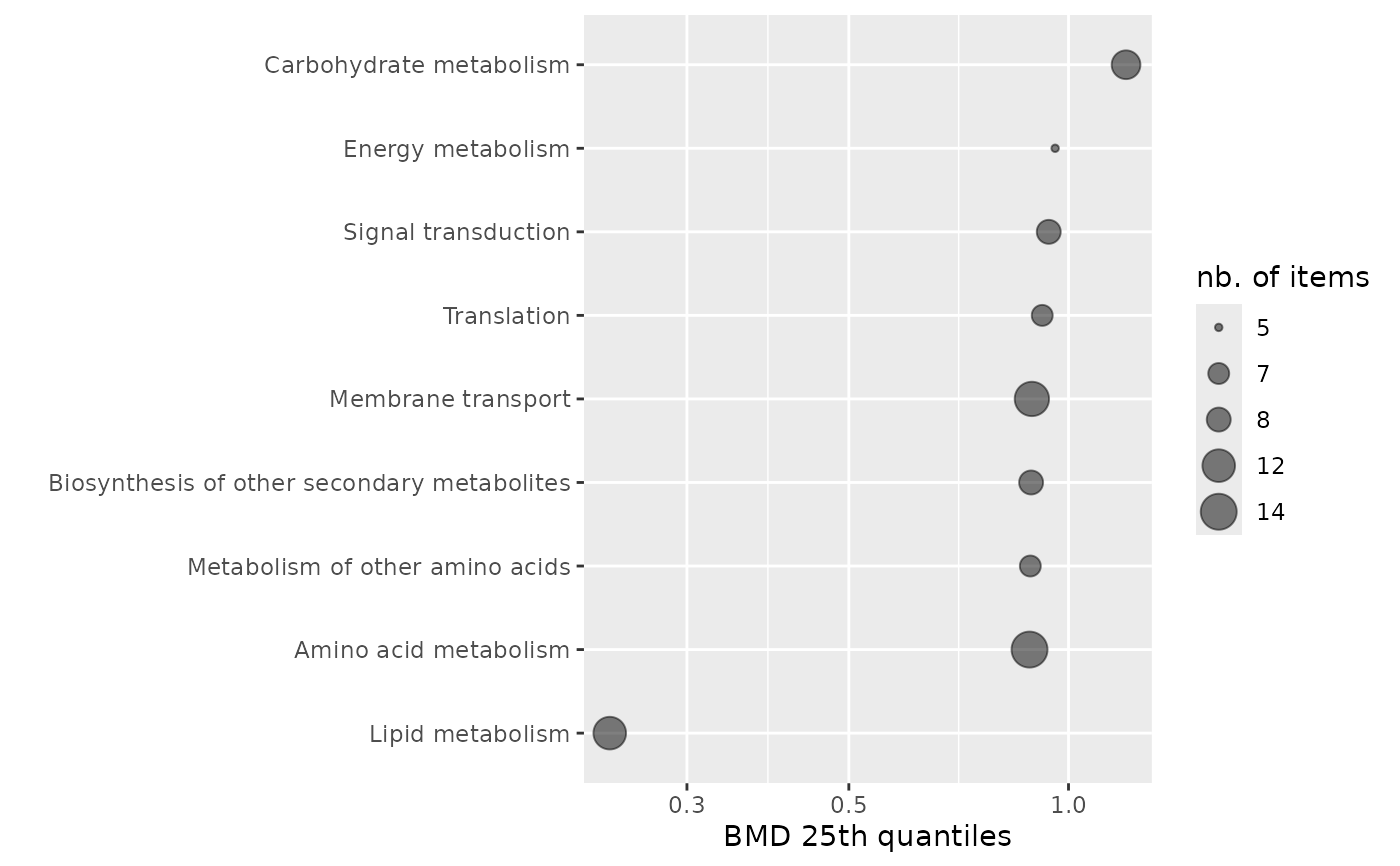
### an ECDFplot of 25th quantiles of BMD-zSD calculated by pathway
sensitivityplot(annotres, BMDtype = "zSD",
group = "path_class",
BMDsummary = "first.quartile")
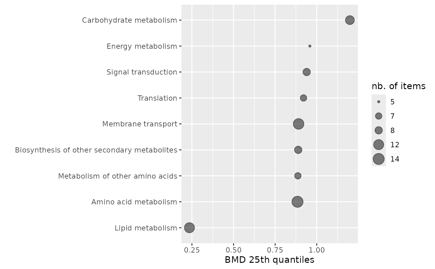
 # \donttest{
# same plot in raw BMD scale (so not in log scale)
sensitivityplot(annotres, BMDtype = "zSD",
group = "path_class",
BMDsummary = "first.quartile",
BMD_log_transfo = FALSE)
# \donttest{
# same plot in raw BMD scale (so not in log scale)
sensitivityplot(annotres, BMDtype = "zSD",
group = "path_class",
BMDsummary = "first.quartile",
BMD_log_transfo = FALSE)
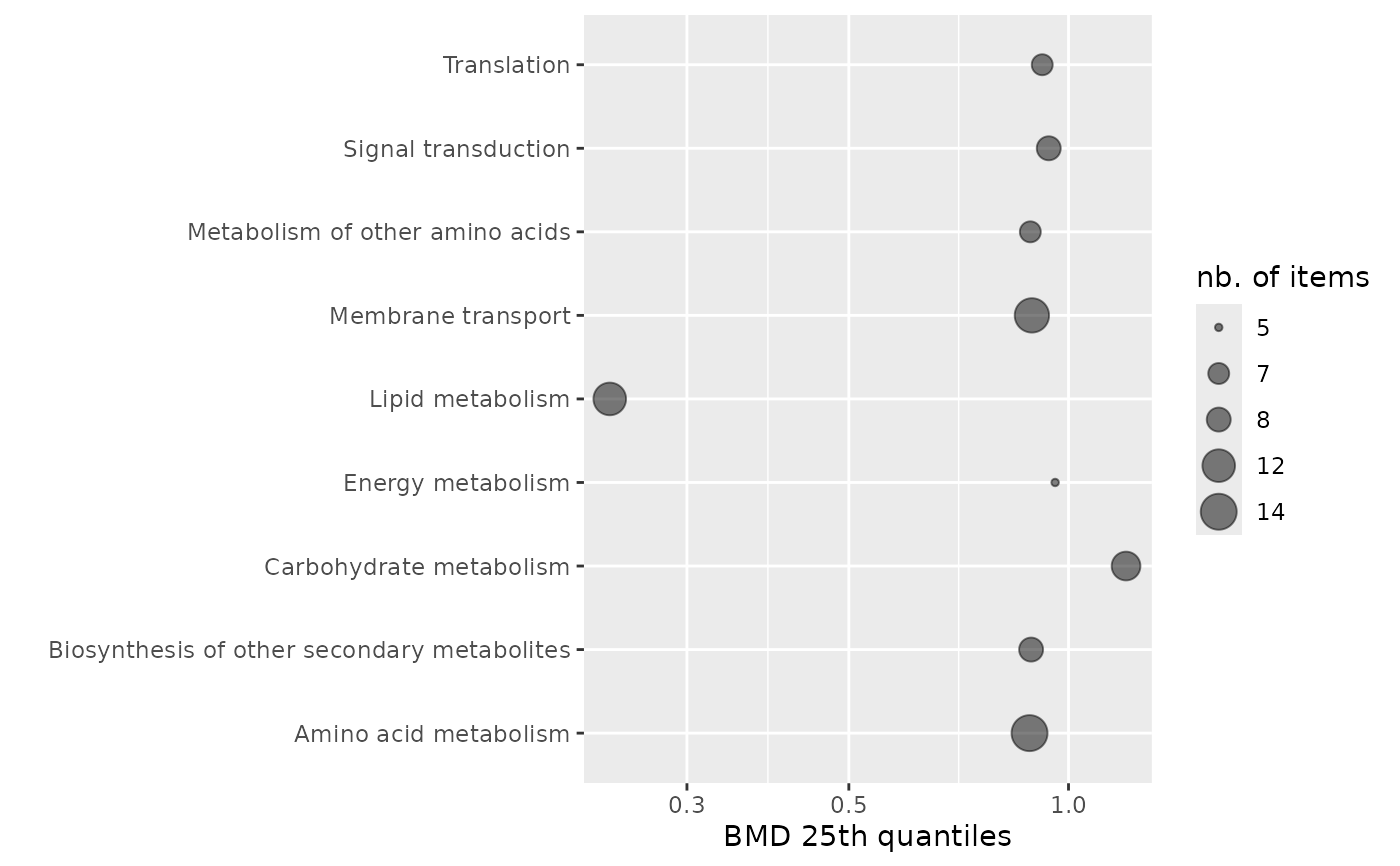
 ### Plot of 25th quantiles of BMD-zSD calculated by pathway
### in the order of the levels as defined in the group input
levels(annotres$path_class)
#> [1] "Amino acid metabolism"
#> [2] "Biosynthesis of other secondary metabolites"
#> [3] "Carbohydrate metabolism"
#> [4] "Energy metabolism"
#> [5] "Lipid metabolism"
#> [6] "Membrane transport"
#> [7] "Metabolism of other amino acids"
#> [8] "Signal transduction"
#> [9] "Translation"
sensitivityplot(annotres, BMDtype = "zSD",
group = "path_class", ECDF_plot = FALSE,
BMDsummary = "first.quartile")
### Plot of 25th quantiles of BMD-zSD calculated by pathway
### in the order of the levels as defined in the group input
levels(annotres$path_class)
#> [1] "Amino acid metabolism"
#> [2] "Biosynthesis of other secondary metabolites"
#> [3] "Carbohydrate metabolism"
#> [4] "Energy metabolism"
#> [5] "Lipid metabolism"
#> [6] "Membrane transport"
#> [7] "Metabolism of other amino acids"
#> [8] "Signal transduction"
#> [9] "Translation"
sensitivityplot(annotres, BMDtype = "zSD",
group = "path_class", ECDF_plot = FALSE,
BMDsummary = "first.quartile")
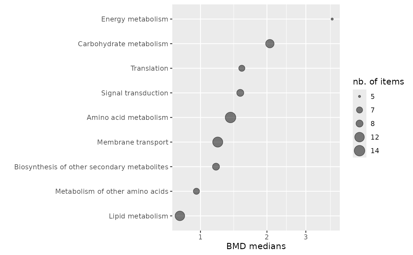
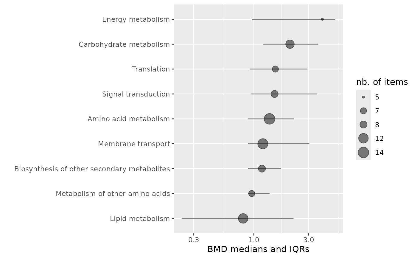
 ### an ECDFplot of medians of BMD-zSD calculated by pathway
sensitivityplot(annotres, BMDtype = "zSD",
group = "path_class",
BMDsummary = "median")
### an ECDFplot of medians of BMD-zSD calculated by pathway
sensitivityplot(annotres, BMDtype = "zSD",
group = "path_class",
BMDsummary = "median")
 ### an ECDFplot of medians of BMD-zSD calculated by pathway
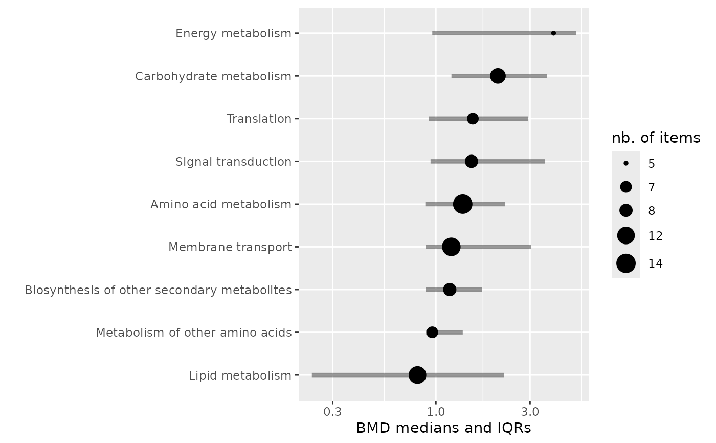
### with addition of interquartile ranges (IQRs)
sensitivityplot(annotres, BMDtype = "zSD",
group = "path_class",
BMDsummary = "median.and.IQR")
### an ECDFplot of medians of BMD-zSD calculated by pathway
### with addition of interquartile ranges (IQRs)
sensitivityplot(annotres, BMDtype = "zSD",
group = "path_class",
BMDsummary = "median.and.IQR")
 ### The same plot playing with graphical parameters
sensitivityplot(annotres, BMDtype = "zSD",
group = "path_class",
BMDsummary = "median.and.IQR",
line.size = 1.5, line.alpha = 0.4, point.alpha = 1)
### The same plot playing with graphical parameters
sensitivityplot(annotres, BMDtype = "zSD",
group = "path_class",
BMDsummary = "median.and.IQR",
line.size = 1.5, line.alpha = 0.4, point.alpha = 1)
 # (2)
# An example with two molecular levels
#
### Rename metabolomic results
metabextendedres <- annotres
# Import the dataframe with transcriptomic results
contigresfilename <- system.file("extdata", "triclosanSVcontigres.txt", package = "DRomics")
contigres <- read.table(contigresfilename, header = TRUE, stringsAsFactors = TRUE)
str(contigres)
#> 'data.frame': 447 obs. of 27 variables:
#> $ id : Factor w/ 447 levels "c00134","c00276",..: 1 2 3 4 5 6 7 8 9 10 ...
#> $ irow : int 2802 39331 41217 52577 52590 53968 54508 57776 58705 60306 ...
#> $ adjpvalue : num 2.76e-04 9.40e-07 2.89e-06 1.88e-03 1.83e-03 ...
#> $ model : Factor w/ 4 levels "Gauss-probit",..: 3 2 2 2 2 2 3 2 1 3 ...
#> $ nbpar : int 2 3 3 3 3 3 2 3 4 2 ...
#> $ b : num -0.21794 1.49944 1.40817 0.00181 1.48605 ...
#> $ c : num NA NA NA NA NA ...
#> $ d : num 10.9 12.4 12.4 16.4 15.3 ...
#> $ e : num NA -2.2 -2.41 1.15 -2.31 ...
#> $ f : num NA NA NA NA NA ...
#> $ SDres : num 0.417 0.287 0.281 0.145 0.523 ...
#> $ typology : Factor w/ 10 levels "E.dec.concave",..: 7 2 2 4 2 2 7 1 5 8 ...
#> $ trend : Factor w/ 4 levels "U","bell","dec",..: 3 3 3 4 3 3 3 3 1 4 ...
#> $ y0 : num 10.9 12.4 12.4 16.4 15.3 ...
#> $ yrange : num 1.445 1.426 1.319 0.567 1.402 ...
#> $ maxychange : num 1.445 1.426 1.319 0.567 1.402 ...
#> $ xextrem : num NA NA NA NA NA ...
#> $ yextrem : num NA NA NA NA NA ...
#> $ BMD.zSD : num 1.913 0.467 0.536 5.073 1.004 ...
#> $ BMR.zSD : num 10.4 12.1 12.1 16.6 14.8 ...
#> $ BMD.xfold : num 4.98 3.88 5.13 NA NA ...
#> $ BMR.xfold : num 9.77 11.19 11.17 18.05 13.8 ...
#> $ BMD.zSD.lower : num 1.255 0.243 0.282 2.65 0.388 ...
#> $ BMD.zSD.upper : num 2.759 0.825 0.925 5.573 2.355 ...
#> $ BMD.xfold.lower : num 3.94 2.32 2.79 Inf 3.06 ...
#> $ BMD.xfold.upper : num Inf Inf Inf Inf Inf ...
#> $ nboot.successful: int 500 497 495 332 466 469 500 321 260 500 ...
# Import the dataframe with functional annotation (or any other descriptor/category
# you want to use, here KEGG pathway classes)
contigannotfilename <- system.file("extdata", "triclosanSVcontigannot.txt", package = "DRomics")
contigannot <- read.table(contigannotfilename, header = TRUE, stringsAsFactors = TRUE)
str(contigannot)
#> 'data.frame': 562 obs. of 2 variables:
#> $ contig : Factor w/ 447 levels "c00134","c00276",..: 1 2 3 4 5 6 7 8 9 10 ...
#> $ path_class: Factor w/ 17 levels "Amino acid metabolism",..: 3 11 11 15 8 4 3 4 8 2 ...
# Merging of both previous dataframes
contigextendedres <- merge(x = contigres, y = contigannot, by.x = "id", by.y = "contig")
# to see the structure of this dataframe
str(contigextendedres)
#> 'data.frame': 562 obs. of 28 variables:
#> $ id : Factor w/ 447 levels "c00134","c00276",..: 1 2 3 4 5 6 7 8 9 10 ...
#> $ irow : int 2802 39331 41217 52577 52590 53968 54508 57776 58705 60306 ...
#> $ adjpvalue : num 2.76e-04 9.40e-07 2.89e-06 1.88e-03 1.83e-03 ...
#> $ model : Factor w/ 4 levels "Gauss-probit",..: 3 2 2 2 2 2 3 2 1 3 ...
#> $ nbpar : int 2 3 3 3 3 3 2 3 4 2 ...
#> $ b : num -0.21794 1.49944 1.40817 0.00181 1.48605 ...
#> $ c : num NA NA NA NA NA ...
#> $ d : num 10.9 12.4 12.4 16.4 15.3 ...
#> $ e : num NA -2.2 -2.41 1.15 -2.31 ...
#> $ f : num NA NA NA NA NA ...
#> $ SDres : num 0.417 0.287 0.281 0.145 0.523 ...
#> $ typology : Factor w/ 10 levels "E.dec.concave",..: 7 2 2 4 2 2 7 1 5 8 ...
#> $ trend : Factor w/ 4 levels "U","bell","dec",..: 3 3 3 4 3 3 3 3 1 4 ...
#> $ y0 : num 10.9 12.4 12.4 16.4 15.3 ...
#> $ yrange : num 1.445 1.426 1.319 0.567 1.402 ...
#> $ maxychange : num 1.445 1.426 1.319 0.567 1.402 ...
#> $ xextrem : num NA NA NA NA NA ...
#> $ yextrem : num NA NA NA NA NA ...
#> $ BMD.zSD : num 1.913 0.467 0.536 5.073 1.004 ...
#> $ BMR.zSD : num 10.4 12.1 12.1 16.6 14.8 ...
#> $ BMD.xfold : num 4.98 3.88 5.13 NA NA ...
#> $ BMR.xfold : num 9.77 11.19 11.17 18.05 13.8 ...
#> $ BMD.zSD.lower : num 1.255 0.243 0.282 2.65 0.388 ...
#> $ BMD.zSD.upper : num 2.759 0.825 0.925 5.573 2.355 ...
#> $ BMD.xfold.lower : num 3.94 2.32 2.79 Inf 3.06 ...
#> $ BMD.xfold.upper : num Inf Inf Inf Inf Inf ...
#> $ nboot.successful: int 500 497 495 332 466 469 500 321 260 500 ...
#> $ path_class : Factor w/ 17 levels "Amino acid metabolism",..: 3 11 11 15 8 4 3 4 8 2 ...
### Merge metabolomic and transcriptomic results
extendedres <- rbind(metabextendedres, contigextendedres)
extendedres$molecular.level <- factor(c(rep("metabolites", nrow(metabextendedres)),
rep("contigs", nrow(contigextendedres))))
str(extendedres)
#> 'data.frame': 646 obs. of 29 variables:
#> $ id : Factor w/ 478 levels "NAP47_51","NAP_2",..: 1 2 3 4 4 4 4 5 6 7 ...
#> $ irow : int 46 2 21 28 28 28 28 34 38 47 ...
#> $ adjpvalue : num 7.16e-04 6.23e-05 1.11e-05 1.03e-05 1.03e-05 ...
#> $ model : Factor w/ 4 levels "Gauss-probit",..: 3 2 3 3 3 3 3 2 2 4 ...
#> $ nbpar : int 2 3 2 2 2 2 2 3 3 5 ...
#> $ b : num -0.056 0.4598 -0.0595 -0.0451 -0.0451 ...
#> $ c : num NA NA NA NA NA ...
#> $ d : num 7.34 5.94 5.39 7.86 7.86 ...
#> $ e : num NA -1.65 NA NA NA ...
#> $ f : num NA NA NA NA NA ...
#> $ SDres : num 0.1245 0.126 0.0793 0.052 0.052 ...
#> $ typology : Factor w/ 10 levels "E.dec.concave",..: 7 2 7 7 7 7 7 2 2 9 ...
#> $ trend : Factor w/ 4 levels "U","bell","dec",..: 3 3 3 3 3 3 3 3 3 1 ...
#> $ y0 : num 7.34 5.94 5.39 7.86 7.86 ...
#> $ yrange : num 0.435 0.456 0.461 0.35 0.35 ...
#> $ maxychange : num 0.435 0.456 0.461 0.35 0.35 ...
#> $ xextrem : num NA NA NA NA NA ...
#> $ yextrem : num NA NA NA NA NA ...
#> $ BMD.zSD : num 2.224 0.528 1.333 1.154 1.154 ...
#> $ BMR.zSD : num 7.22 5.82 5.31 7.81 7.81 ...
#> $ BMD.xfold : num NA NA NA NA NA ...
#> $ BMR.xfold : num 6.61 5.35 4.85 7.07 7.07 ...
#> $ BMD.zSD.lower : num 0.979 0.2 0.853 0.752 0.752 ...
#> $ BMD.zSD.upper : num 4.07 1.11 1.75 1.46 1.46 ...
#> $ BMD.xfold.lower : num Inf Inf 7.61 Inf Inf ...
#> $ BMD.xfold.upper : num Inf Inf Inf Inf Inf ...
#> $ nboot.successful: int 1000 957 1000 1000 1000 1000 1000 648 620 872 ...
#> $ path_class : Factor w/ 18 levels "Amino acid metabolism",..: 5 5 3 3 2 6 8 5 5 5 ...
#> $ molecular.level : Factor w/ 2 levels "contigs","metabolites": 2 2 2 2 2 2 2 2 2 2 ...
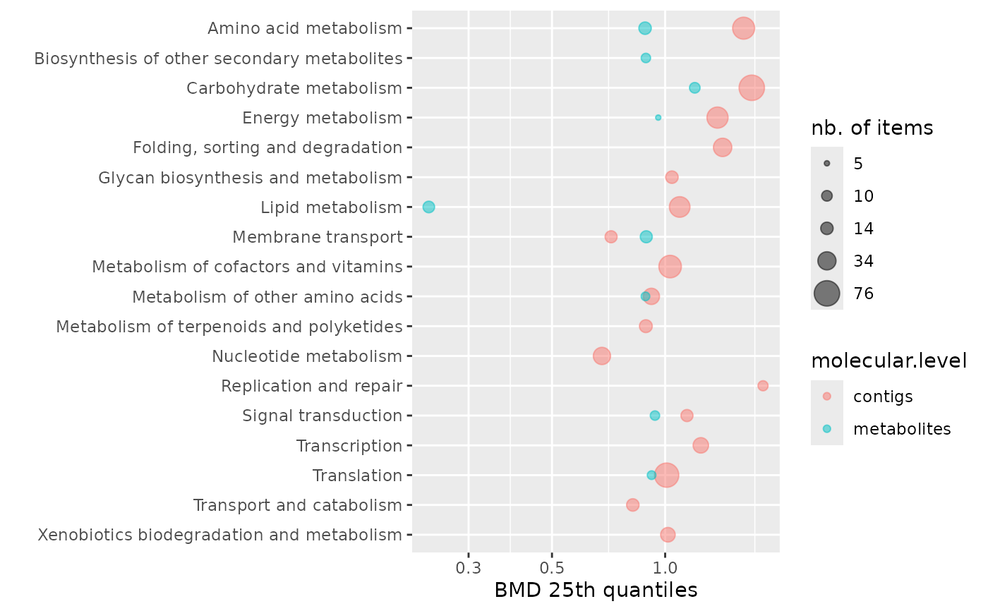
### Plot of 25th quantiles of BMD-zSD calculated by pathway
### and colored by molecular level
# optional inverse alphabetic ordering of groups for the plot
extendedres$path_class <- factor(extendedres$path_class,
levels = sort(levels(extendedres$path_class),
decreasing = TRUE))
sensitivityplot(extendedres, BMDtype = "zSD",
group = "path_class", colorby = "molecular.level",
BMDsummary = "first.quartile")
# (2)
# An example with two molecular levels
#
### Rename metabolomic results
metabextendedres <- annotres
# Import the dataframe with transcriptomic results
contigresfilename <- system.file("extdata", "triclosanSVcontigres.txt", package = "DRomics")
contigres <- read.table(contigresfilename, header = TRUE, stringsAsFactors = TRUE)
str(contigres)
#> 'data.frame': 447 obs. of 27 variables:
#> $ id : Factor w/ 447 levels "c00134","c00276",..: 1 2 3 4 5 6 7 8 9 10 ...
#> $ irow : int 2802 39331 41217 52577 52590 53968 54508 57776 58705 60306 ...
#> $ adjpvalue : num 2.76e-04 9.40e-07 2.89e-06 1.88e-03 1.83e-03 ...
#> $ model : Factor w/ 4 levels "Gauss-probit",..: 3 2 2 2 2 2 3 2 1 3 ...
#> $ nbpar : int 2 3 3 3 3 3 2 3 4 2 ...
#> $ b : num -0.21794 1.49944 1.40817 0.00181 1.48605 ...
#> $ c : num NA NA NA NA NA ...
#> $ d : num 10.9 12.4 12.4 16.4 15.3 ...
#> $ e : num NA -2.2 -2.41 1.15 -2.31 ...
#> $ f : num NA NA NA NA NA ...
#> $ SDres : num 0.417 0.287 0.281 0.145 0.523 ...
#> $ typology : Factor w/ 10 levels "E.dec.concave",..: 7 2 2 4 2 2 7 1 5 8 ...
#> $ trend : Factor w/ 4 levels "U","bell","dec",..: 3 3 3 4 3 3 3 3 1 4 ...
#> $ y0 : num 10.9 12.4 12.4 16.4 15.3 ...
#> $ yrange : num 1.445 1.426 1.319 0.567 1.402 ...
#> $ maxychange : num 1.445 1.426 1.319 0.567 1.402 ...
#> $ xextrem : num NA NA NA NA NA ...
#> $ yextrem : num NA NA NA NA NA ...
#> $ BMD.zSD : num 1.913 0.467 0.536 5.073 1.004 ...
#> $ BMR.zSD : num 10.4 12.1 12.1 16.6 14.8 ...
#> $ BMD.xfold : num 4.98 3.88 5.13 NA NA ...
#> $ BMR.xfold : num 9.77 11.19 11.17 18.05 13.8 ...
#> $ BMD.zSD.lower : num 1.255 0.243 0.282 2.65 0.388 ...
#> $ BMD.zSD.upper : num 2.759 0.825 0.925 5.573 2.355 ...
#> $ BMD.xfold.lower : num 3.94 2.32 2.79 Inf 3.06 ...
#> $ BMD.xfold.upper : num Inf Inf Inf Inf Inf ...
#> $ nboot.successful: int 500 497 495 332 466 469 500 321 260 500 ...
# Import the dataframe with functional annotation (or any other descriptor/category
# you want to use, here KEGG pathway classes)
contigannotfilename <- system.file("extdata", "triclosanSVcontigannot.txt", package = "DRomics")
contigannot <- read.table(contigannotfilename, header = TRUE, stringsAsFactors = TRUE)
str(contigannot)
#> 'data.frame': 562 obs. of 2 variables:
#> $ contig : Factor w/ 447 levels "c00134","c00276",..: 1 2 3 4 5 6 7 8 9 10 ...
#> $ path_class: Factor w/ 17 levels "Amino acid metabolism",..: 3 11 11 15 8 4 3 4 8 2 ...
# Merging of both previous dataframes
contigextendedres <- merge(x = contigres, y = contigannot, by.x = "id", by.y = "contig")
# to see the structure of this dataframe
str(contigextendedres)
#> 'data.frame': 562 obs. of 28 variables:
#> $ id : Factor w/ 447 levels "c00134","c00276",..: 1 2 3 4 5 6 7 8 9 10 ...
#> $ irow : int 2802 39331 41217 52577 52590 53968 54508 57776 58705 60306 ...
#> $ adjpvalue : num 2.76e-04 9.40e-07 2.89e-06 1.88e-03 1.83e-03 ...
#> $ model : Factor w/ 4 levels "Gauss-probit",..: 3 2 2 2 2 2 3 2 1 3 ...
#> $ nbpar : int 2 3 3 3 3 3 2 3 4 2 ...
#> $ b : num -0.21794 1.49944 1.40817 0.00181 1.48605 ...
#> $ c : num NA NA NA NA NA ...
#> $ d : num 10.9 12.4 12.4 16.4 15.3 ...
#> $ e : num NA -2.2 -2.41 1.15 -2.31 ...
#> $ f : num NA NA NA NA NA ...
#> $ SDres : num 0.417 0.287 0.281 0.145 0.523 ...
#> $ typology : Factor w/ 10 levels "E.dec.concave",..: 7 2 2 4 2 2 7 1 5 8 ...
#> $ trend : Factor w/ 4 levels "U","bell","dec",..: 3 3 3 4 3 3 3 3 1 4 ...
#> $ y0 : num 10.9 12.4 12.4 16.4 15.3 ...
#> $ yrange : num 1.445 1.426 1.319 0.567 1.402 ...
#> $ maxychange : num 1.445 1.426 1.319 0.567 1.402 ...
#> $ xextrem : num NA NA NA NA NA ...
#> $ yextrem : num NA NA NA NA NA ...
#> $ BMD.zSD : num 1.913 0.467 0.536 5.073 1.004 ...
#> $ BMR.zSD : num 10.4 12.1 12.1 16.6 14.8 ...
#> $ BMD.xfold : num 4.98 3.88 5.13 NA NA ...
#> $ BMR.xfold : num 9.77 11.19 11.17 18.05 13.8 ...
#> $ BMD.zSD.lower : num 1.255 0.243 0.282 2.65 0.388 ...
#> $ BMD.zSD.upper : num 2.759 0.825 0.925 5.573 2.355 ...
#> $ BMD.xfold.lower : num 3.94 2.32 2.79 Inf 3.06 ...
#> $ BMD.xfold.upper : num Inf Inf Inf Inf Inf ...
#> $ nboot.successful: int 500 497 495 332 466 469 500 321 260 500 ...
#> $ path_class : Factor w/ 17 levels "Amino acid metabolism",..: 3 11 11 15 8 4 3 4 8 2 ...
### Merge metabolomic and transcriptomic results
extendedres <- rbind(metabextendedres, contigextendedres)
extendedres$molecular.level <- factor(c(rep("metabolites", nrow(metabextendedres)),
rep("contigs", nrow(contigextendedres))))
str(extendedres)
#> 'data.frame': 646 obs. of 29 variables:
#> $ id : Factor w/ 478 levels "NAP47_51","NAP_2",..: 1 2 3 4 4 4 4 5 6 7 ...
#> $ irow : int 46 2 21 28 28 28 28 34 38 47 ...
#> $ adjpvalue : num 7.16e-04 6.23e-05 1.11e-05 1.03e-05 1.03e-05 ...
#> $ model : Factor w/ 4 levels "Gauss-probit",..: 3 2 3 3 3 3 3 2 2 4 ...
#> $ nbpar : int 2 3 2 2 2 2 2 3 3 5 ...
#> $ b : num -0.056 0.4598 -0.0595 -0.0451 -0.0451 ...
#> $ c : num NA NA NA NA NA ...
#> $ d : num 7.34 5.94 5.39 7.86 7.86 ...
#> $ e : num NA -1.65 NA NA NA ...
#> $ f : num NA NA NA NA NA ...
#> $ SDres : num 0.1245 0.126 0.0793 0.052 0.052 ...
#> $ typology : Factor w/ 10 levels "E.dec.concave",..: 7 2 7 7 7 7 7 2 2 9 ...
#> $ trend : Factor w/ 4 levels "U","bell","dec",..: 3 3 3 3 3 3 3 3 3 1 ...
#> $ y0 : num 7.34 5.94 5.39 7.86 7.86 ...
#> $ yrange : num 0.435 0.456 0.461 0.35 0.35 ...
#> $ maxychange : num 0.435 0.456 0.461 0.35 0.35 ...
#> $ xextrem : num NA NA NA NA NA ...
#> $ yextrem : num NA NA NA NA NA ...
#> $ BMD.zSD : num 2.224 0.528 1.333 1.154 1.154 ...
#> $ BMR.zSD : num 7.22 5.82 5.31 7.81 7.81 ...
#> $ BMD.xfold : num NA NA NA NA NA ...
#> $ BMR.xfold : num 6.61 5.35 4.85 7.07 7.07 ...
#> $ BMD.zSD.lower : num 0.979 0.2 0.853 0.752 0.752 ...
#> $ BMD.zSD.upper : num 4.07 1.11 1.75 1.46 1.46 ...
#> $ BMD.xfold.lower : num Inf Inf 7.61 Inf Inf ...
#> $ BMD.xfold.upper : num Inf Inf Inf Inf Inf ...
#> $ nboot.successful: int 1000 957 1000 1000 1000 1000 1000 648 620 872 ...
#> $ path_class : Factor w/ 18 levels "Amino acid metabolism",..: 5 5 3 3 2 6 8 5 5 5 ...
#> $ molecular.level : Factor w/ 2 levels "contigs","metabolites": 2 2 2 2 2 2 2 2 2 2 ...
### Plot of 25th quantiles of BMD-zSD calculated by pathway
### and colored by molecular level
# optional inverse alphabetic ordering of groups for the plot
extendedres$path_class <- factor(extendedres$path_class,
levels = sort(levels(extendedres$path_class),
decreasing = TRUE))
sensitivityplot(extendedres, BMDtype = "zSD",
group = "path_class", colorby = "molecular.level",
BMDsummary = "first.quartile")
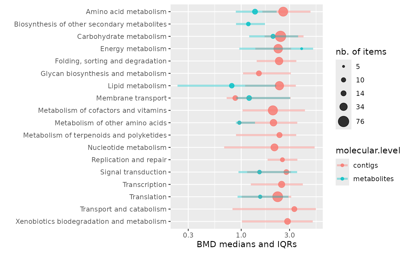
 ### Plot of medians and IQRs of BMD-zSD calculated by pathway
### and colored by molecular level
sensitivityplot(extendedres, BMDtype = "zSD",
group = "path_class", colorby = "molecular.level",
BMDsummary = "median.and.IQR",
line.size = 1.2, line.alpha = 0.4,
point.alpha = 0.8)
### Plot of medians and IQRs of BMD-zSD calculated by pathway
### and colored by molecular level
sensitivityplot(extendedres, BMDtype = "zSD",
group = "path_class", colorby = "molecular.level",
BMDsummary = "median.and.IQR",
line.size = 1.2, line.alpha = 0.4,
point.alpha = 0.8)
 # }
# }